1. Introduction
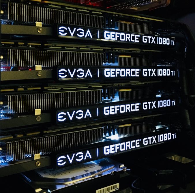
At Parkopedia’s Autonomous Valet Parking team, we will be creating indoor car park maps for autonomous vehicles. Throughout this 2.5 year project, in collaboration with Transport System Catapult and the University of Surrey, we expect to be doing a significant amount of deep learning. We estimate that over the course of this project there will be intensive training on large datasets, for multiple days, weeks or even more. As any deep learning project there are three distinct phases in the research and development pipeline, which can be loosely described as (1) prototyping; (2) hyperparameter search and (3) intensive training. While there will be a lot of prototyping involved, which we believe any high-end desktop computer equipped with one GTX Nvidia 1080 Ti will fit our needs, the next question is how do we efficiently solve (2) and (3). Typically, in (2) one picks different parameters of the model and trains it against the dataset (or part of it) for a few iterations. In our case, a reasonable estimate could be perhaps 10 different runs, each taking a day of processing time. This insight (best hyperparameters) is then used to apply heavy computation in (3).
We are at the early stages of this project, but due to accounting reasons, we need to have a clear vision now on where we want to apply the budget for computing power for deep learning. Given that we know beforehand that we’ll need to have it for a relatively long period and we will do a lot of experimentation on large amounts of data, we want to investigate what is the most cost effective solution. On the other hand, because of the high processing times involved, it is important that the solution has enough flexibility to the research team, in that heavy computation times don’t hinder the ability to focus on other tasks that might require a GPU too. This blog post is about finding the sweet spot between these two.
The discussion is generally around on-premise hardware vs cloud based solutions. A cloud based solution is appealing because resources are readily available, maintenance-free, and one can launch as many computing machines as desired at any point in time. This flexibility also has a much wider hardware choice: a multitude of flavours are available so one is not restricted to working with a certain hardware architecture. Of course, these very interesting features come with a price. Whilst an office-based solution doesn’t offer these characteristics, it is interesting to see how they compare, especially in the long run. Therefore, it comes down to asking the following question:
What infrastructure gives us the best compromise between time-to-solution, cost-to-solution and availability of the resources ?
The goal of this document is to do a performance vs cost study on different possible architectures, both cloud-based and office-based. We ran benchmarks on various AWS GPU instances, and extrapolated some of the results to other similar cloud based architectures on Google Cloud. We compared the results against a system with 4 Nvidia GTX 1080 Tis, by extrapolating the results obtained for a single GTX 1080 Ti, which we currently have. An analysis was made both in terms of performance and cost.
2. Experimental Setup
We ran the tensorflow benchmark code repository which according to their description, “contains implementations of several popular convolutional models, and is designed to be as fast as possible. tf_cnn_benchmarks supports both running on a single machine or running in distributed mode across multiple hosts.”, which is perfect for running it against various infrastructures, both in single and multiple GPU scenarios. In terms of software all the infractures had the exact same configuration, namely:
- Cudnn 7.1.4
- Cuda 9.0
- Python 2.7
- Ubuntu 16.04
2.1. Amazon Web Services (AWS)
Amazon’s GPU options are very simple: you choose an instance which comes with one (or more) GPUs of any given type. We compared three GPU families on AWS p2s (K80s), g3s (M60s) and p3s (V100s).
| Gpu | Instance | #GPUs | On demand price $/hour | 1 day | 1 week | 1 month |
| NVIDIA K80 | p2.xlarge | 1 | 0.9 | 21.6 | 151.2 | 658.8 |
| p2.8xlarge | 8 | 7.2 | 172.8 | 1209.6 | 5270.4 | |
| p2.16xlarge | 16 | 14.4 | 345.6 | 2419.2 | 10540.8 | |
| Tesla M60 | g3.4xlarge | 1 | 1.14 | 27.36 | 191.52 | 834.48 |
| g3.8xlarge | 2 | 2.28 | 54.72 | 383.04 | 1668.96 | |
| g3.16xlarge | 4 | 4.56 | 109.44 | 766.08 | 3337.92 | |
| NVIDIA V100 | p3.2xlarge | 1 | 3.06 | 73.44 | 514.08 | 2239.92 |
| p3.8xlarge | 4 | 12.24 | 293.76 | 2056.32 | 8959.68 | |
| p3.16xlarge | 8 | 24.48 | 587.52 | 4112.64 | 17919.36 |
2.2. EC2 Spot Instances
Spot instances are a solution offered by Amazon’s EC2, which defines it as an: “(…) unused EC2 instance that is available for less than the On-Demand price. Because Spot Instances enable you to request unused EC2 instances at steep discounts, you can lower your Amazon EC2 costs significantly (…)”. One thing to have in mind is that its pricing scheme is based on offer/demand model, resulting in a fluctuant hourly rate. In a nutshell, the user selects the hardware (say p3.2xlarge), defines how much he/she is willing to pay per hour, and the machine is accessible, provided the price set is below AWS’ price threshold. In such an event, the machine is automatically shutdown by Amazon. On the financial side, this is obviously very appealing as one gets the same hardware for a fraction of the cost. However, on the technical side, this solution requires a more complex architecture, which can handle interruptions (on a DL scenario this means most likely saving the network’s weights and gradients often to a location outside the local instance). The user must also accept downtimes – even if there is an orchestration mechanism that automatically launches on-demand instances to recover the loss of an instance and continue training/inference, there’s an initialization stage (setting up the instance, downloading the last state of the network, downloading the dataset, etc) – that cannot be ignored. Moreover, there’s a considerable effort in coming up with such orchestration mechanism, which cannot be disregarded as well, as it brings to advantages to the deep learning researcher; in fact, it’s quite the opposite.
Because of these reasons, this solution doesn’t directly compare with the two main solutions in debate. Nevertheless, we believe that in order to have a more balanced post, it should be added here. Below is a screenshot of the last 3 months obtained from AWS’ EC2 Management Console for a p2.8xlarge instance.
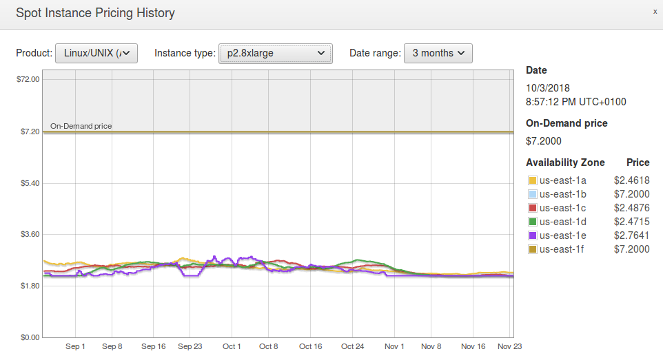
In order to work out an hourly rate for EC2 spot instances, we’ve taken the cheapest curve for all the availability zones, and we came up with a ballpark estimate for its average price throughout the 3 months period. The following table summarizes this information for all the instances, as well as the discount with respect to the on demand prices.
| Spot price
$/hour |
Cost
wrt on-demand |
||
| p2.xlarge | 0.28 | 31% | |
| p2.8xlarge | 2.71 | 38% | |
| p2.16xlarge | 5.32 | 37% | |
| g3.4xlarge | 0.37 | 32% | |
| g3.8xlarge | 0.68 | 30% | |
| g3.16xlarge | 1.37 | 30% | |
| p3.2xlarge | 1.11 | 36% | |
| p3.8xlarge | 4.85 | 40% | |
| p3.16xlarge | 8.00 | 33% |
2.2. Office GPU box
For a proper comparison against cloud-based solutions, we need to come up with an hourly rate for the office GPU. Working out the equivalent price/hour involves making assumptions on the utilization (the more we use it, the cheaper it becomes, per hour). In addition to the hardware acquisition, we want a maintenance contract. This is because we want to minimize downtimes when a certain GPU goes out of order temporarily (unfortunately, it is not that unusual, and is in itself a disadvantage of this solution). Because this project will run for 30 months, we can amortize this price per month and depending on the average utilization in terms of the number of days the box is used (24 hours per day, uninterruptedly), we can reach a final figure for the hourly rate. To be even fairer, one might consider adding in the electricity costs, which we thought it would make sense.
Broadly speaking, in our scenario, a box of 4 x GTX 1080 Ti (about $6.5k USD with a maintenance contract), assuming 20 USD cents per kwh in the UK, being used 10 days per month equates into about $1.30/hour. We appreciate this 10 days is a strong assumption, especially in this early stages of the project. Therefore we test different utilization figures later. A breakdown of this figures is shown below:
| Cost estimation of office GPUs | |
| Hardware | |
| Box (4*1080tis) | $6,500.00 |
| w/ 5 Year Warranty, 3 Years Collect & Return | |
| Total Acquisition Cost | $6,500.00 |
| Amortization | |
| Months (length of project) | 30 |
| Price / month | $216.67 |
| Electricity | |
| Price per kwh | 0.2 |
| Utilization (days per month running 24/7) | 10 |
| Cost / month | $48.00 |
| Global cost / month | $264.67 |
| Cost/hour
(assuming previous utilization) |
1.10 |
2.3. Google Compute Engine (GCE)
Google Cloud’s model is slightly different than AWS’ model, in that GPUs are attached to an instance, so one can combine a certain GPU with different host characteristics. As per Google Cloud’s pricing page: “Each GPU adds to the cost of your instance in addition to the cost of the machine type”. We did not run any benchmarks on google cloud, but because their prices are different we thought it would make sense to add GCE’s scenario. Because of this, we only took into account hardware setups that would be comparable to the AWS’ offer, in terms of the GPUs.
Their GPU offering for GPUs consists on the following boards: NVIDIA Tesla V100, NVIDIA Tesla K80 and NVIDIA Tesla P100. The latter was discarded as there’s no counterpart on aws. Also, regarding the K80’s one can only select 1,2,4 and 8 GPUs and as for the NVIDIA V100’s, only 1 or 8 GPUs can be selected
In order to obtain a similar instance to those in AWS, we selected the “base instances” so that the number of vCPUs is the same, as follows:
| Alias | Instance | GPUs | Price/h ($) [first term is the instance price/h] |
Equivalent aws instance |
| GCE_1xV100 | n1-standard-8 | 1xV100 | 0.38+2.48 = 2.86 | p3.2xlarge |
| GCE_8xV100 | n1-standard-64 | 8xV100 | 3.04+8*2.48 = 22.88 | p3.16xlarge |
| GCE_1xK80 | n1-standard-4 | 1xK80 | 0.04+0.45 = 0.49 | p2.xlarge |
| GCE_8xK80 | n1-standard-32 | 8xK80 | 1.52+8*0.45 = 5.12 | p2.8xlarge |
In terms of performance benchmarks, Tensorflow has done this comparison already. Amazon’s p2.8xlarge was compared against a similar instance, which we denote as GCE_8xK80. Although there appears to be a minor difference, the results are approximately similar, as expected. In our context, we believe we can safely assume the same for the three remaining cases, so we simply used the same performance metrics.
We also took Google TPUs into account. This blog post compared AWS’ p3.8xlarge against a cloud TPU. They show that on ResNet50 with a batch size of 1024 (the recommended size by Google), the TPU device is slightly faster, but slower at any other smaller batch size. We omitted this fact, and used our measurements obtained on the p3.8xlarge.
3. Performance Results
We ran the benchmark code in three different standard models (Inception3, VGG16 and ResNet50) using three different batch sizes per GPU: 16, 32 and 64, meaning that in a multi-GPU training session the effective global number of images per batch is #GPUs x batch size. Half-precision computation was used. A typical command line call would look like this:
python tf_cnn_benchmarks.py --num_gpus=1 --batch_size=16 --model=resnet50 --use_fp16
As per TensorFlow’s performance guide, “obtaining optimal performance on multi-GPUs is a challenge” […] “How each tower gets the updated variables and how the gradients are applied has an impact on the performance, scaling, and convergence of the mode”. As mentioned earlier, the goal of this analysis is to obtain a ballpark estimate on cloud vs on-premise in terms of performance and cost, so gpu-related optimization issues, are out of scope of this post (this issue has been addressed in various other blog posts, e.g. see: Towards Efficient Multi-GPU Training in Keras with TensorFlow). That said, when we ran the benchmarking code with its default configuration (as show in the python command above), we soon realised we were having poor scalability in terms of throughput, i.e. the throughput didn’t scale well with the number of GPUs, so that wouldn’t be a fair comparison in a more optimized scenario. After reading Tensorflow’s tips, and a bit of experimentation we reached a setup which we were happy with. Note also that using different gpu optimizations might have an impact on training convergence, but we will ignore that for the remainder of this post. Despite this, we only fined-tuned g3.16xlarge and p2.16xlarge and p3.16xlarge instances, which was where the scalability issues were seriously being noted. Note that we don’t claim this to be by any means the optimum configuration, nor did we put serious efforts in it, but it allows us to make a more coherent comparison. The table below shows the scaling efficiency obtained after optimizing each of the three multi-GPU instances, with respect to the respective instance that has a single GPU. For each configuration (AWS instance / model ) the associated letter (A, B, C, x ) refers to the configuration in use, as follows:
A : variable_update:replicated | nccl:no | local_parameter_device:cpu
B : variable_update:replicated | nccl:yes | local_parameter_device:gpu
C : variable_update:replicated | nccl:no | local_parameter_device:gpu
x - default configuration
| Inception3 | ResNet50 | VGG16 | |||||||||||
| #GPU | Config | 16 | 32 | 64 | 16 | 32 | 64 | 16 | 32 | 64 | |||
| 2 | g3.4xlarge -> g3.8xlarge | x | 0.94 | 0.96 | 0.97 | x | 0.93 | 0.95 | 0.97 | x | 0.84 | 0.89 | 0.93 |
| 4 | g3.4xlarge -> g3.16xlarge | A | 0.94 | 0.96 | 0.96 | A | 0.92 | 0.96 | 0.97 | B | 0.87 | 0.92 | 0.93 |
| 8 | p2.xlarge -> p2.8xlarge | x | 0.90 | 0.88 | 0.87 | x | 0.89 | 0.89 | 0.90 | x | 0.70 | 0.87 | 0.92 |
| 16 | p2.xlarge -> p2.16xlarge | C | 0.74 | 0.81 | 0.86 | A | 0.58 | 0.77 | 0.84 | C | 0.39 | 0.52 | 0.64 |
| 4 | p3.2xlarge -> p3.8xlarge | x | 0.72 | 0.75 | 0.81 | x | 0.73 | 0.78 | 0.83 | x | 0.65 | 0.74 | 0.83 |
| 8 | p3.2xlarge -> p3.16xlarge | B | 0.57 | 0.64 | 0.72 | B | 0.53 | 0.60 | 0.68 | B | 0.55 | 0.66 | 0.78 |
| Average | 0.80 | 0.83 | 0.87 | 0.76 | 0.83 | 0.87 | 0.67 | 0.77 | 0.84 | ||||
In the perfect world these numbers would all be close to 1.0, showing a perfectly linear efficiency in terms of performance as the number of GPUs scale from 1 to many. This table shows that scaling is not perfect but some setups can get quite close.
As mentioned in the introduction, we have one GTX 1080 Ti where we can run these tests on, therefore we had to estimate the performance figures on a box with four of these GPUs. We simply used the average obtained in the earlier table for each of the datasets and batch sizes (see row in red). We believed this to be a relatively conservative estimate. These are the figures obtained.
| Inception3 | ResNet50 | VGG16 | |||||||||
| 16 | 32 | 64 | 16 | 32 | 64 | 16 | 32 | 64 | |||
| 1×1080 Ti | 136 | 145 | 160 | 213 | 250 | 273 | 118 | 137 | 149 | ||
| 4×1080 Tis** | 435 | 482 | 556 | 649 | 825 | 947 | 314 | 418 | 498 | ||
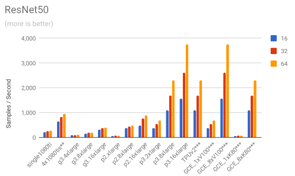
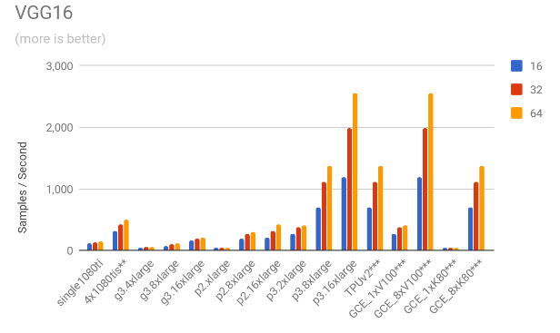
3.1. Throughput comparison
The following charts show the samples / second for each of the models for all the mentioned scenarios.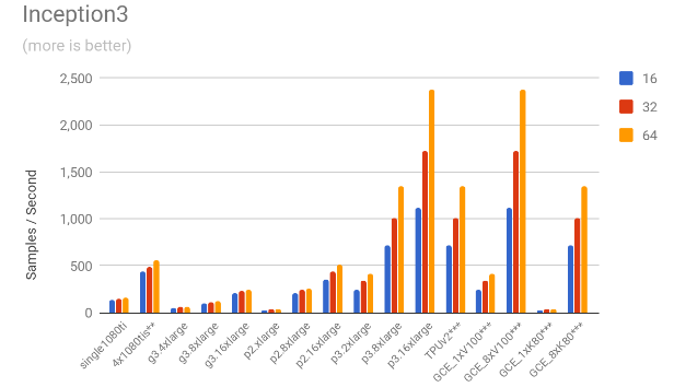
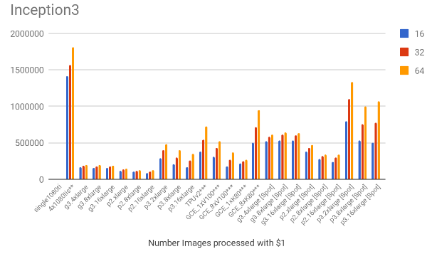
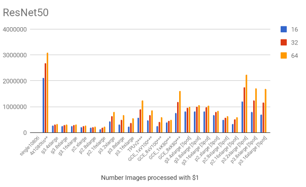
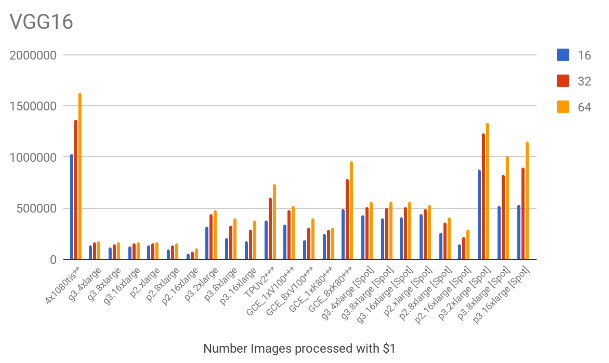
4. Cost results
Based on the throughput and the hourly costs we can estimate the number of images we can process with $1, which is shown below. Note that the EC2 spot prices were also included on these charts.
5. Additional Comparisons
5.1. ILSVRC
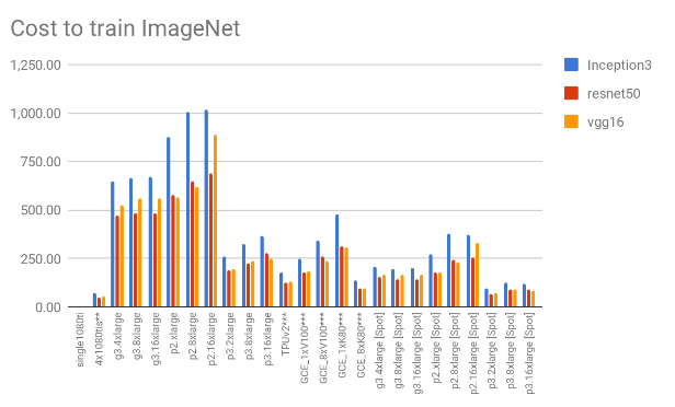
We don’t know yet the amount of data we will be processing, so we thought the ImageNet dataset would be a good choice to give us some real-world intuition on what to expect in terms of time to train and global cost in dollars, as it is pretty much the “industry standard” in deep learning and also because of its respectful size. For each of the models, we their respective papers give us the batch size and the number of iterations, which allows us to work out the total number of samples seen when training.
| Inception3 | ResNet50 | VGG16 | |
| Paper | https://arxiv.org/pdf/1512.00567.pdf | https://arxiv.org/pdf/1512.03385v1.pdf | https://arxiv.org/pdf/1409.1556v6.pdf |
| Batch size | 1600 | 256 | 256 |
| Iterations | 80000 | 600000 | 370000 |
| Total number of samples seen | 128,000,000 | 153,600,000 | 94,720,000 |
To estimate these figures, we simply used the cost and time for a batch of 64 for all the models. Note however that in reality the figures would be lower (both for the time and consequently, the cost). This is because we are using a smaller batch size in our estimations, so a better utilisation of the GPU memory (bigger batch size) would increase the performance, so this is just for illustration purposes. Of course, this choice would impact convergence, but we’re disregarding that too.
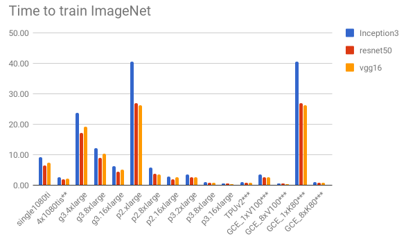
The two charts below shows us the cost and time to train. Considering only “persistent” solutions (all except EC2 Spot instances), the office-based solution offers a much cheaper solution – almost 2x cheaper than the Google’s GCE_8xK80 (the cheapest persistent cloud-based solution). It is still about 36% cheaper than the cheapest solution on the “spot instances” model. Another interesting fact is that it is the forth best performing solution in terms of time to train.
5.2. Gain vs utilization
On previous estimates, we were using an utilisation figure of 10 days – running the box on average 240h per month. As this is just a guess, it is interesting to know how much do we gain (or lose) as we change the number of days per month when compared to a cloud-based solution. To simplify we’ve compared different utilisations against the three best scenarios on VGG16 (64). Again, by doing this comparison on VGG16, is itself a conservative choice, as out of all the models, VGG16 is the one where the images/cost gain of 4x1080tis versus the second best scenario (GCE_8xK80) is smaller – it is better by only approximately 1.7x versus 1.9x on ResNet50 and Inception3, on batch sizes of 64. The comparison is shown on the chart below.
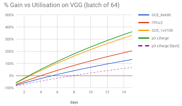
Out of all the the persistent solutions, Google’s GCE_8xK80 is clearly the one with the best value for money. Yet, after 5 days of usage per month, the office GPU outbids Google’s all other cloud based instances. After about 8.5 days per month the box is twice as cheap as TPUv2 – 1.8x and 1.9x respectively for p3.x2large and p3.8xlarge instances. This increases slightly to 10 days for GCE_8xK80. The cheapest spot instance price get outbid only after 8 days of continuous usage.
6. Closing remarks
We believe that throughout our analysis, we were highly conservative in the estimates for an office GPU machine. Essentially, when assumptions had to be made, we tried to compare an office based solution against worst performing scenarios. An accurate estimate depends a lot on the actual scenario but here we tried to be slightly pessimistic with regards to an office based solution.
What we believe matters most is the time and cost to reach a certain solution and our analysis on ILSVRC shows that the 4xGTX1080tis lies perfectly on the sweet spot between these two factors. Another interesting angle is the utilisation chart which clearly shows that, if a GPU box will be used for slightly more than 5 days per month, then cost wise, the on-premise solution is the clear winner. So, on long projects such as the one we’re about to embark, an office based solution is a no-brainer. Therefore the choice is mostly obvious if you need to use GPUs extensively.
Nethertheless, we would like to highlight the following points:
- In terms of costs, when compared to AWS, Google’s cloud GPU offering is worth investigating.
- We are mindful EC2 spot instances are very appealing, but we believe this scenario didn’t fit our purposes because to gain the value from spot instances a maximum price needs to be set and the job will be terminated if that threshold is breached. Even if it its drawbacks can be surpassed using additional logic to handle the termination and re-start of instances gracefully, we believe such configuration is non-optimal and wouldn’t be appropriate for us.
- Another point for consideration regarding EC2 spot prices is that although this analysis was done over a relatively long period of 3 months, effectively reducing the fluctuations, there’s no guarantee cost will stay more or less fixed in the future. In the best scenario it can even be lower, but predictability is required in when budgeting for a 2.5 year project.
Recent Comments