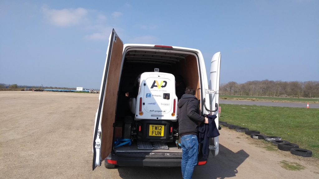
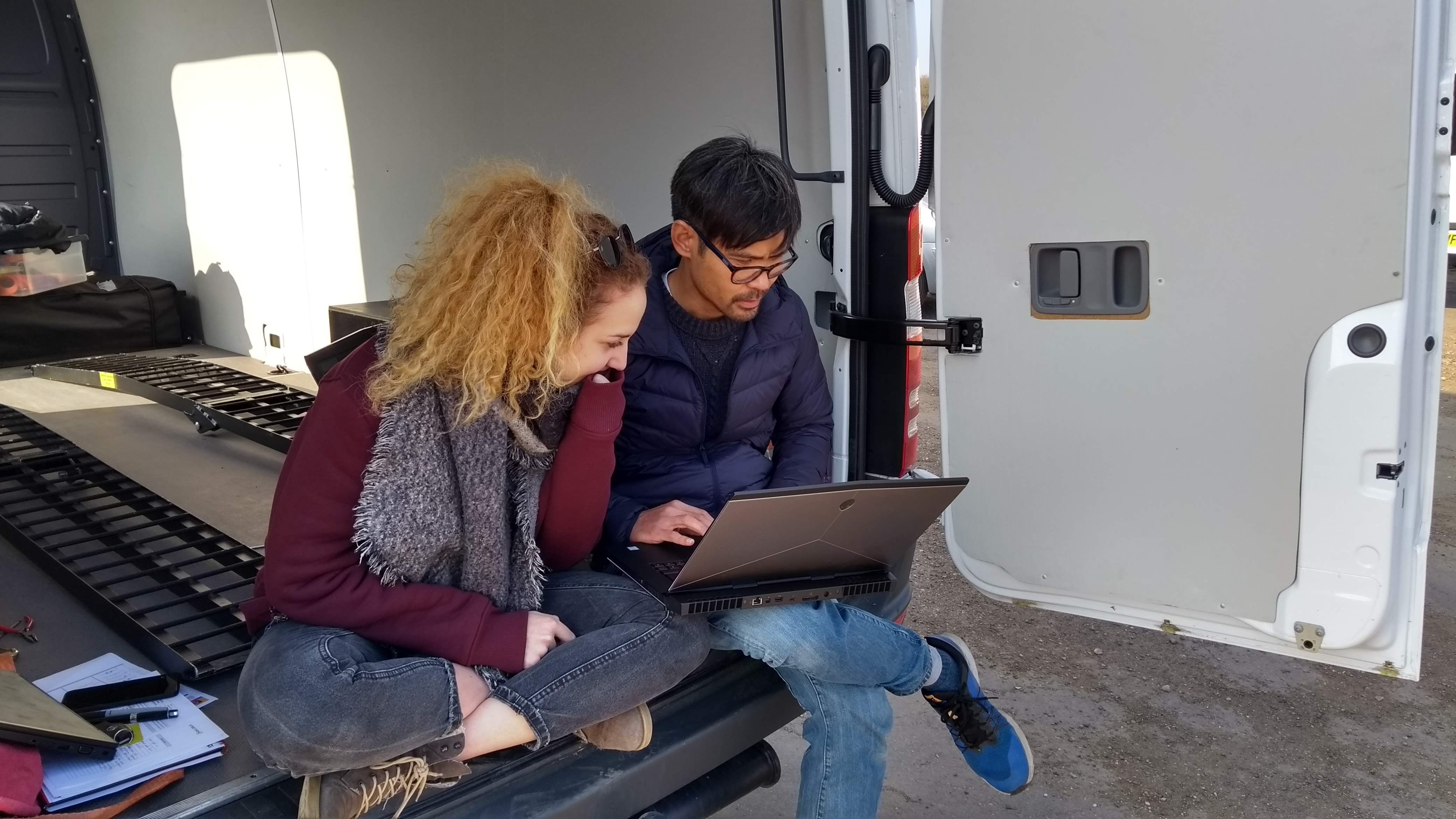
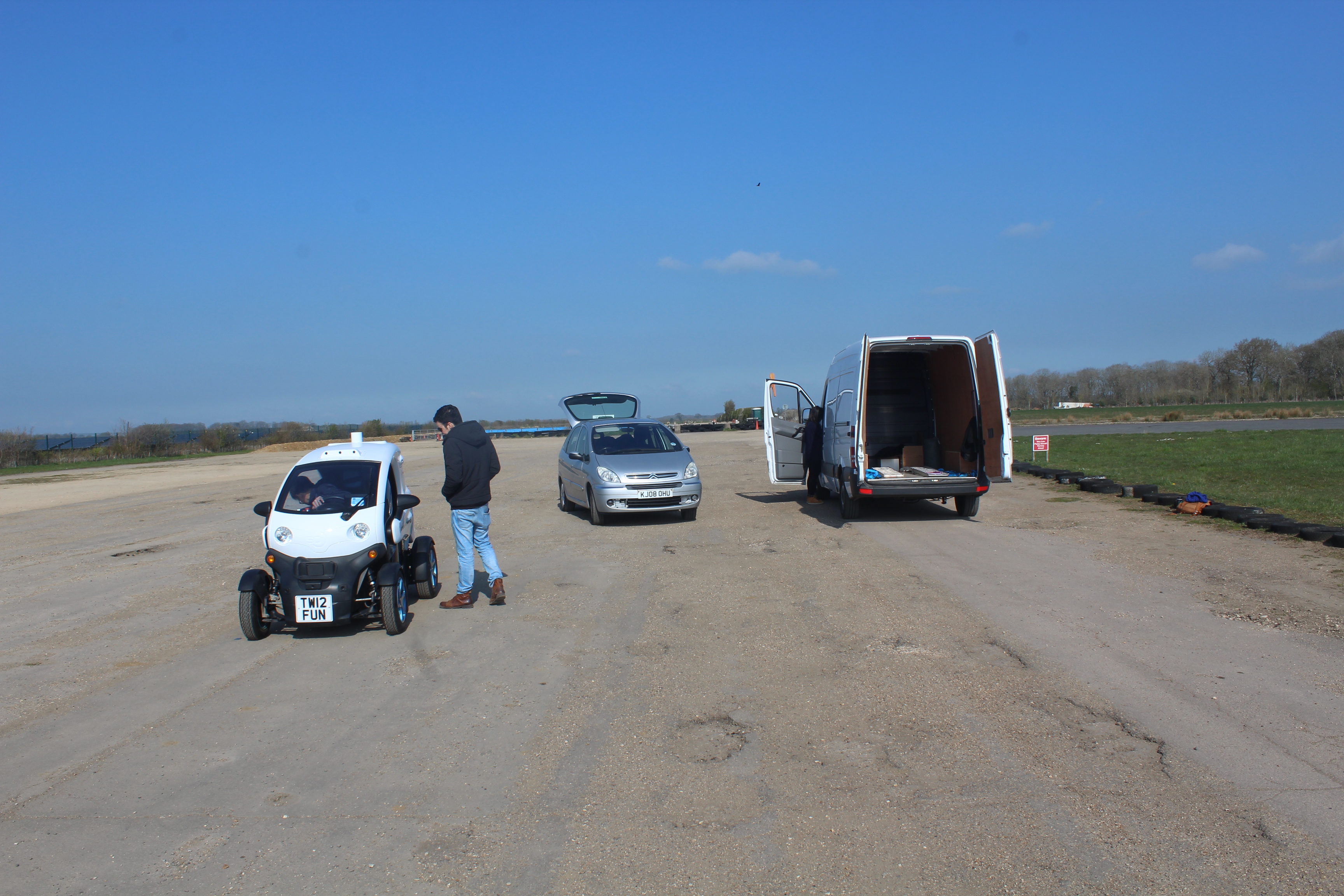
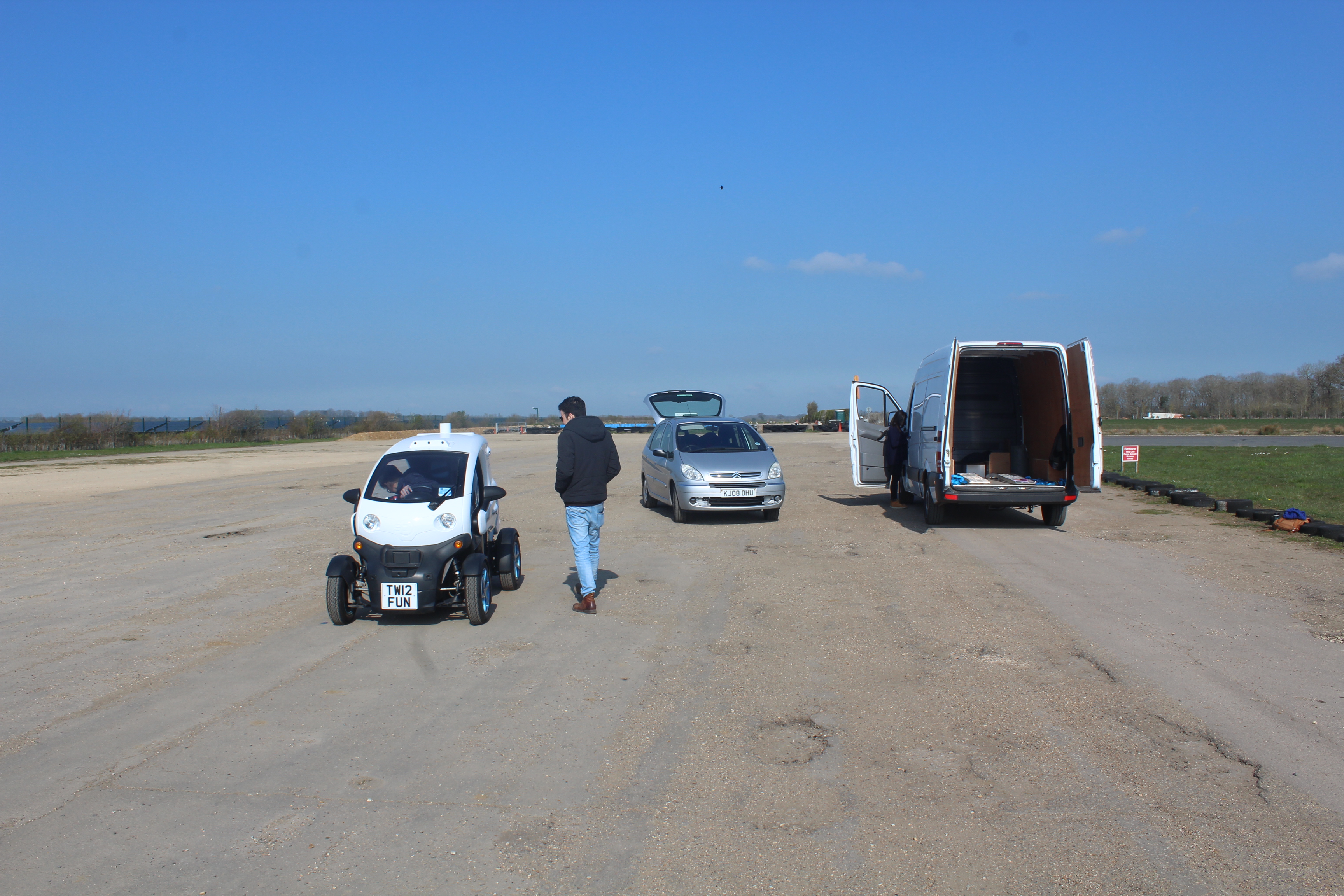
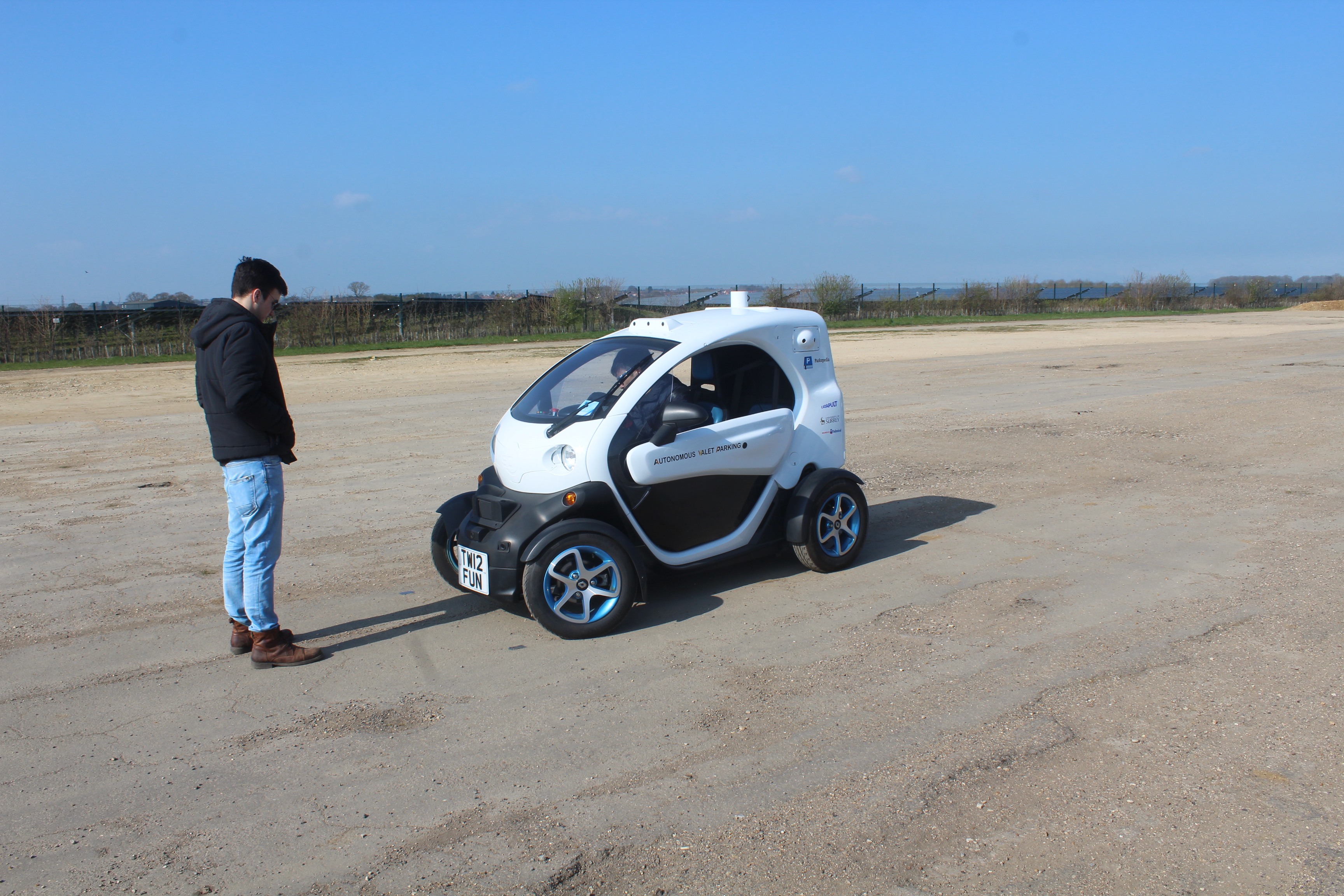
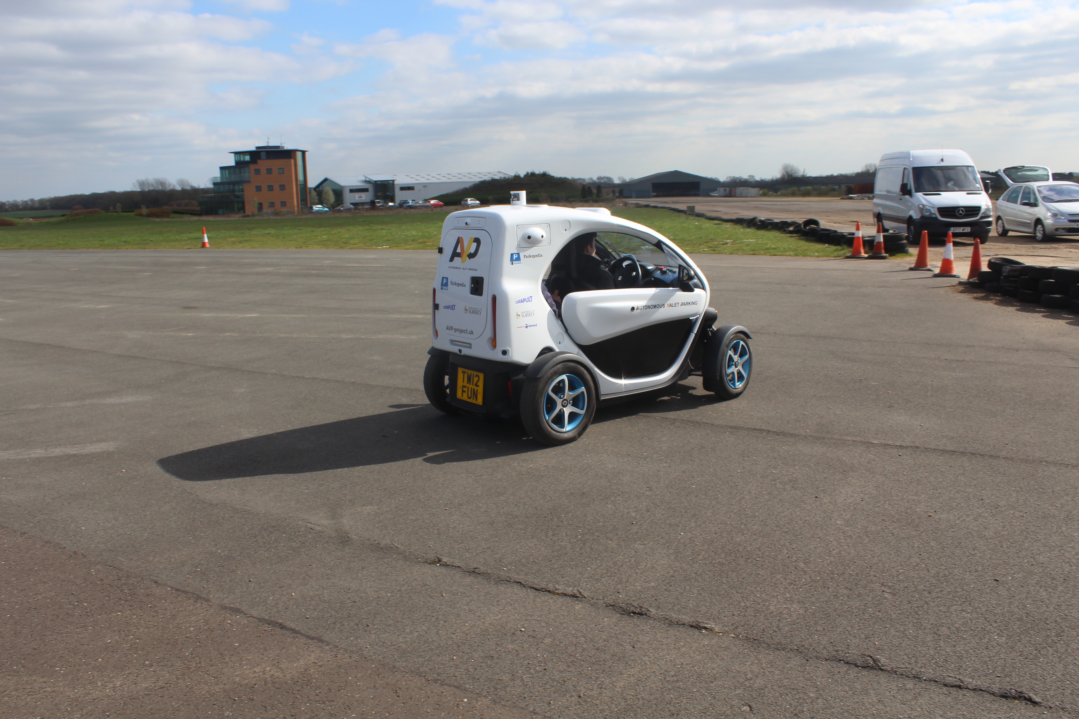
We successfully completed our first tests at Turweston Aerodrome last week.
Unloading the StreetDrone.ONE
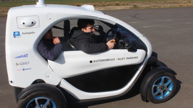
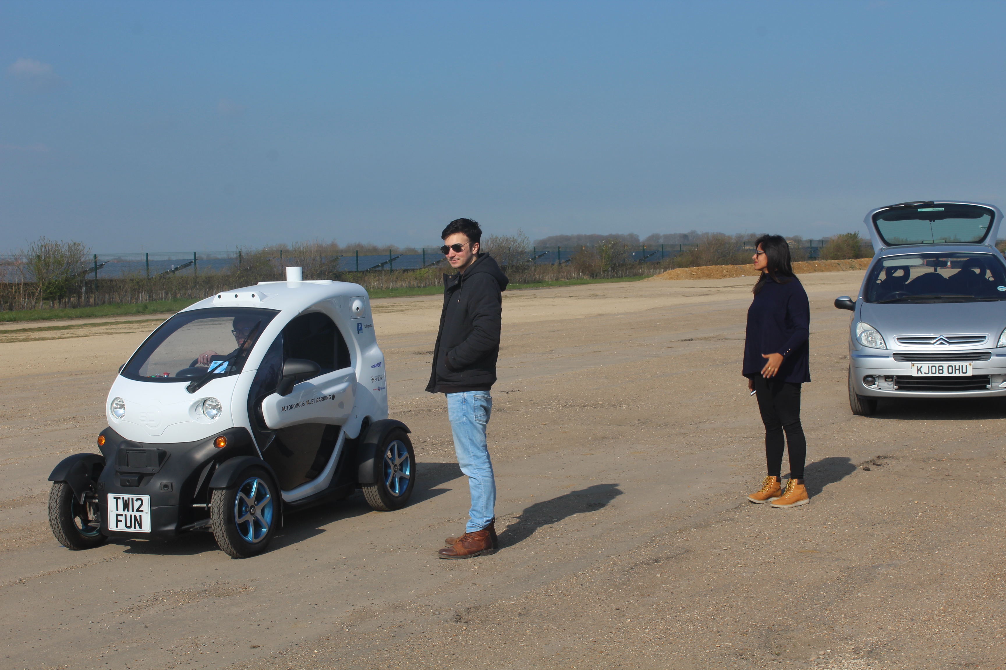
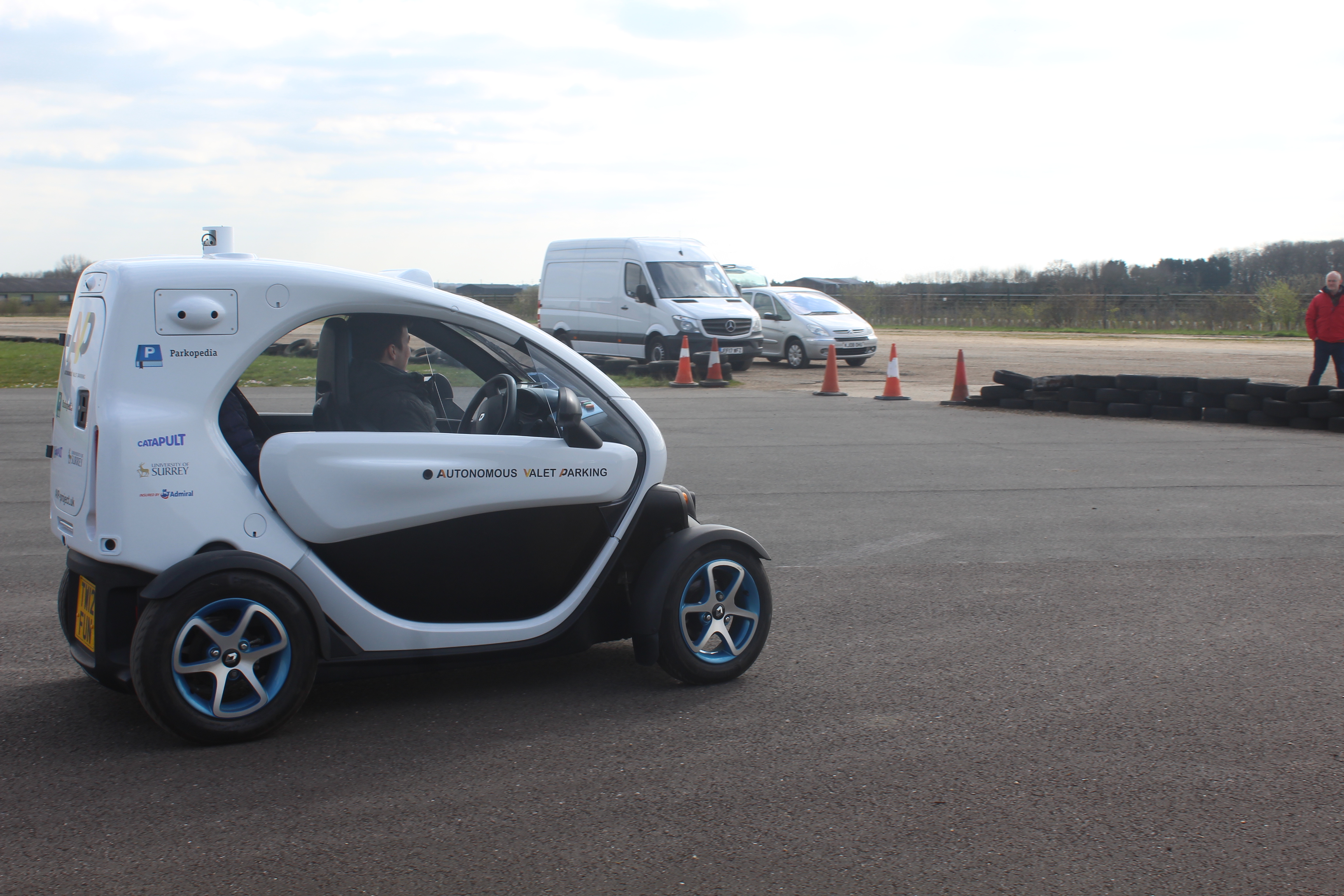
The plan was to check and ensure the robustness of the drive-by-wire system, to train our safety drivers and to do basic path following.
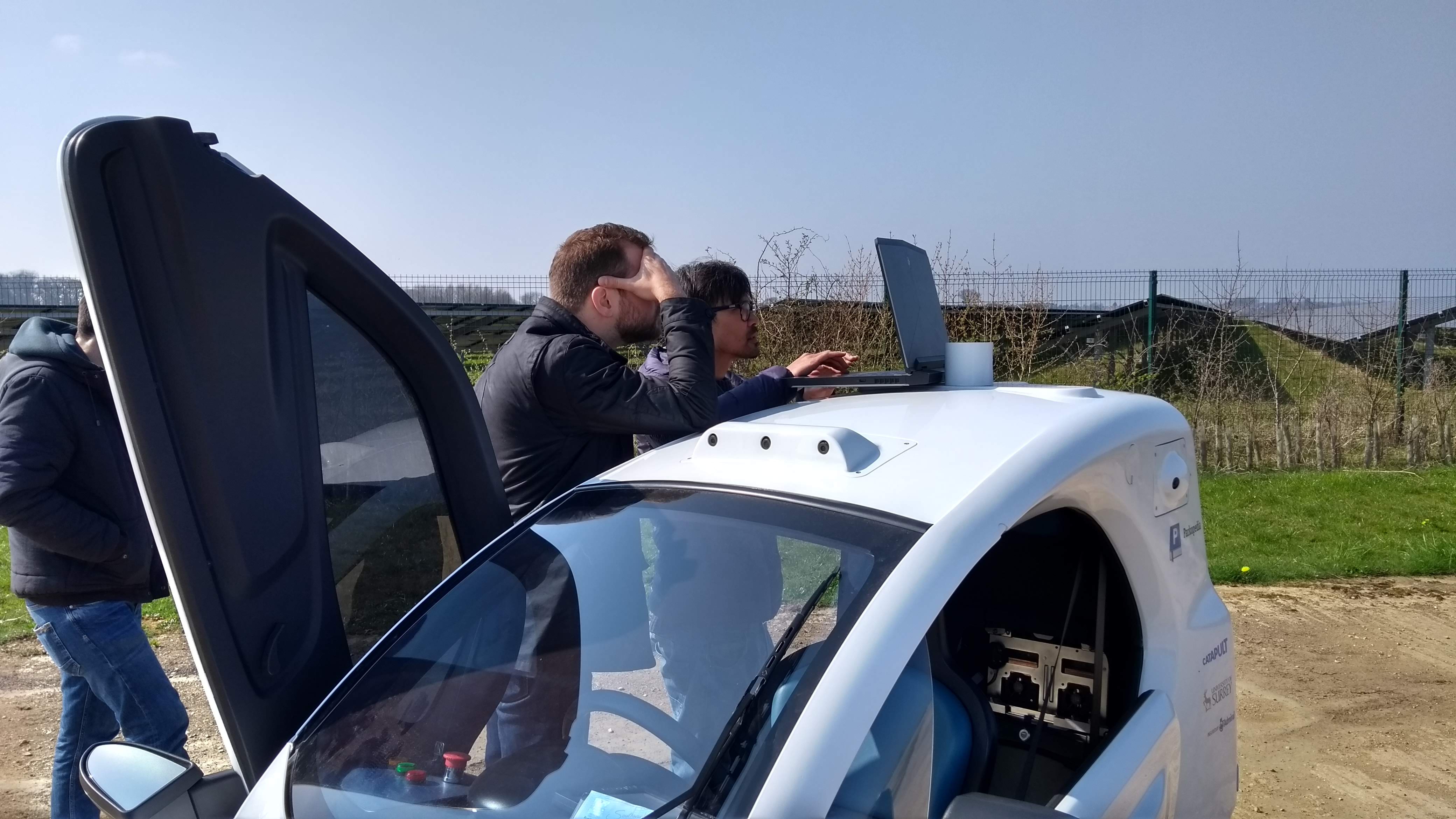
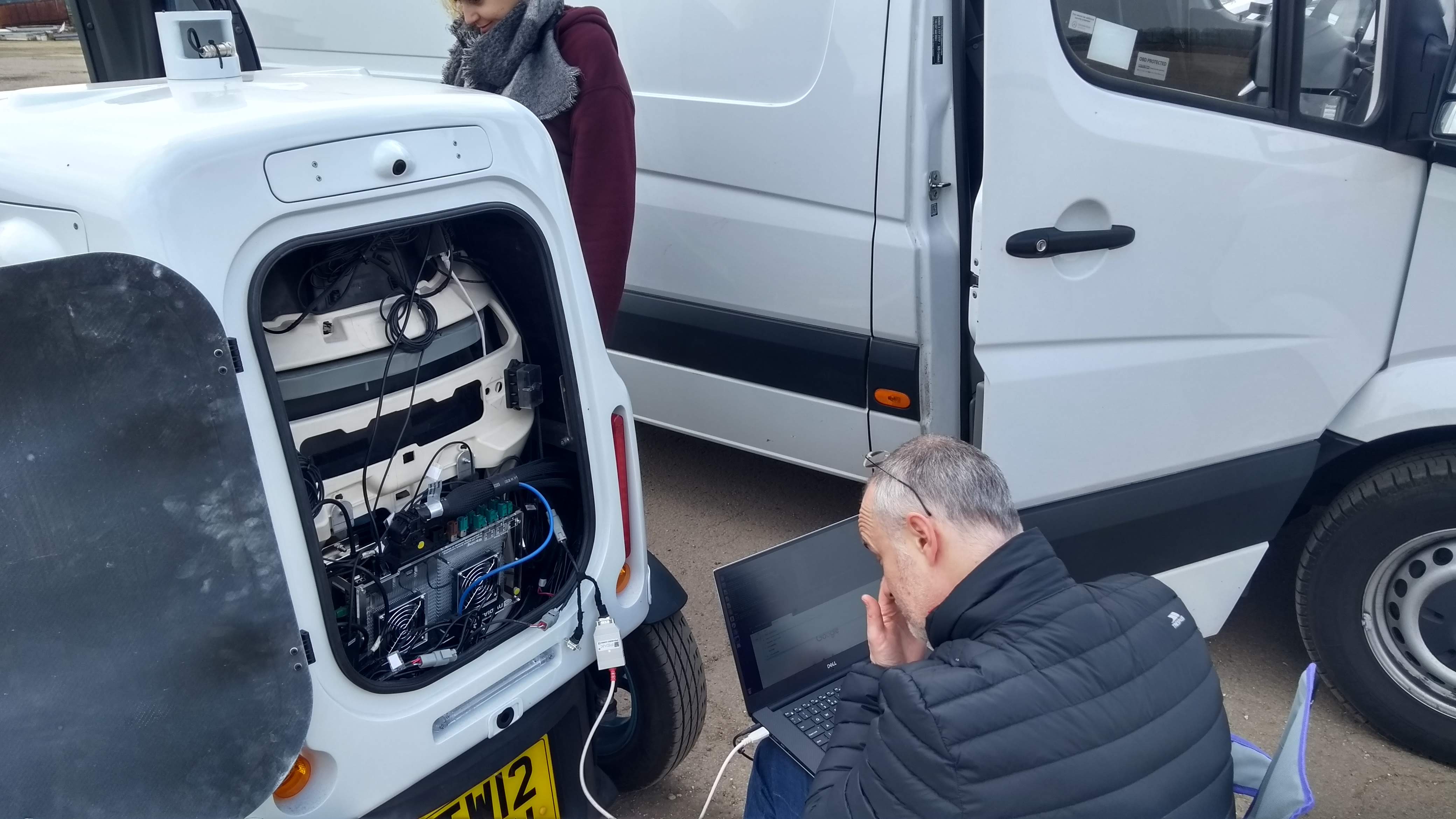
We also took the opportunity to collect some data from the ultrasonic sensors that are on the StreetDrone.ONE which we will use for system safety.
Ultrasonic data collectionDrive-by-wire testing
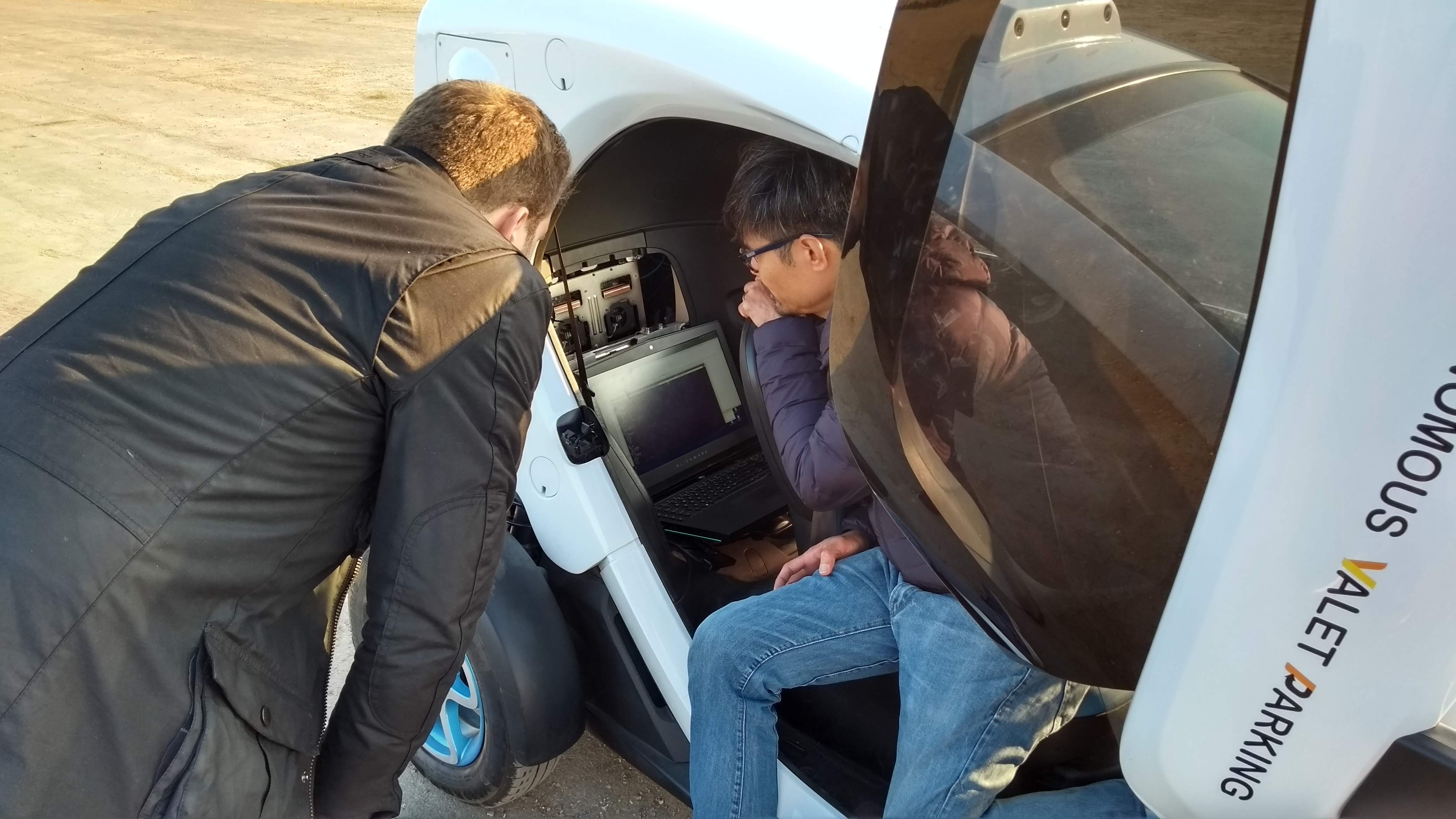
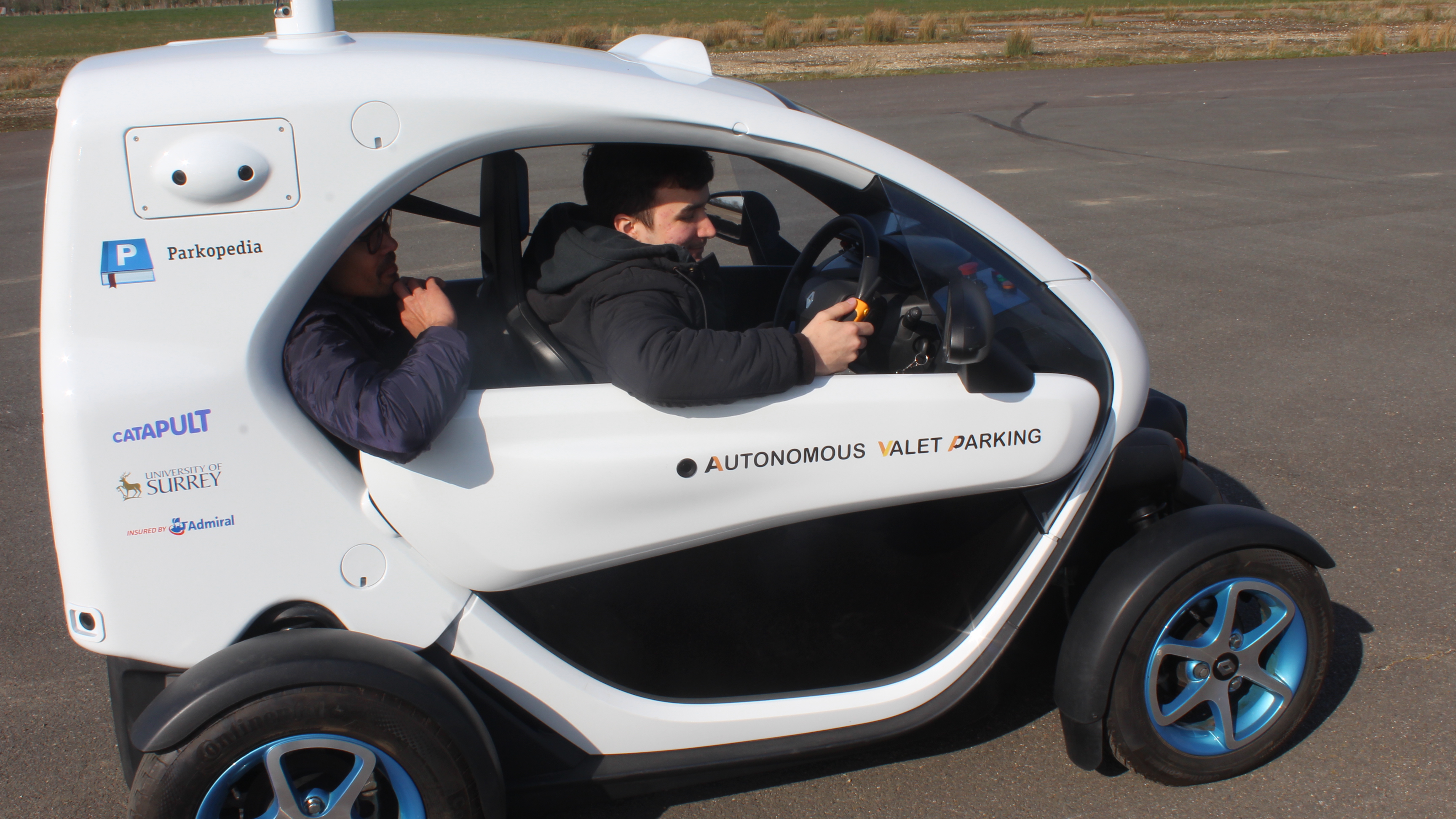
For testing the drive-by-wire system, we carried out a number of test runs using teleoperation from the driver. We drove on the track forward, backward and changing steering at various speeds. The system performed satisfactorily. We also performed a full brake test to work out a safe driving speed and stopping distance in a case of emergency stop. Further details are presented in this blog post.
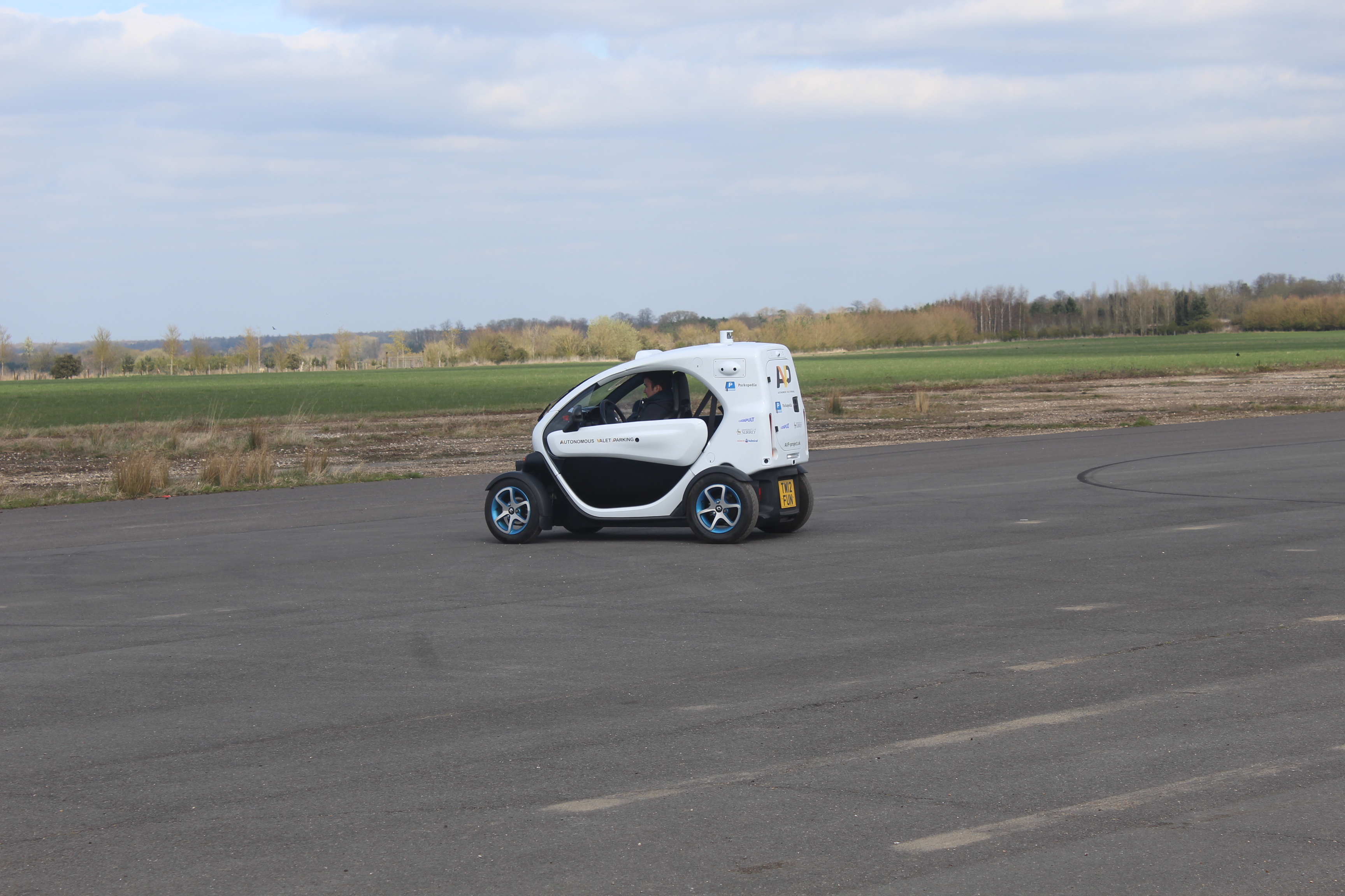
Path following with PID feedback control and a basic GPS and IMU localisation
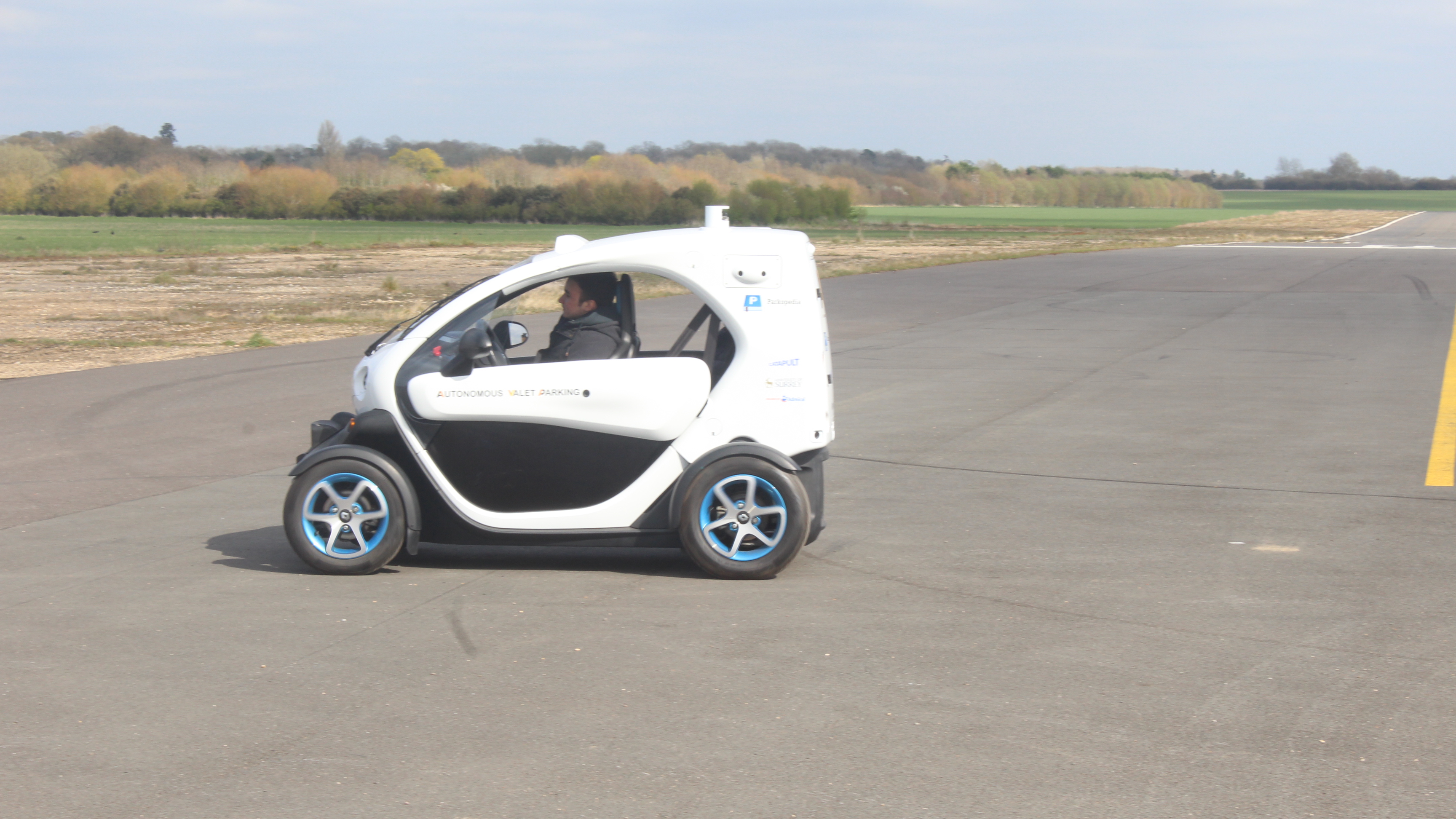
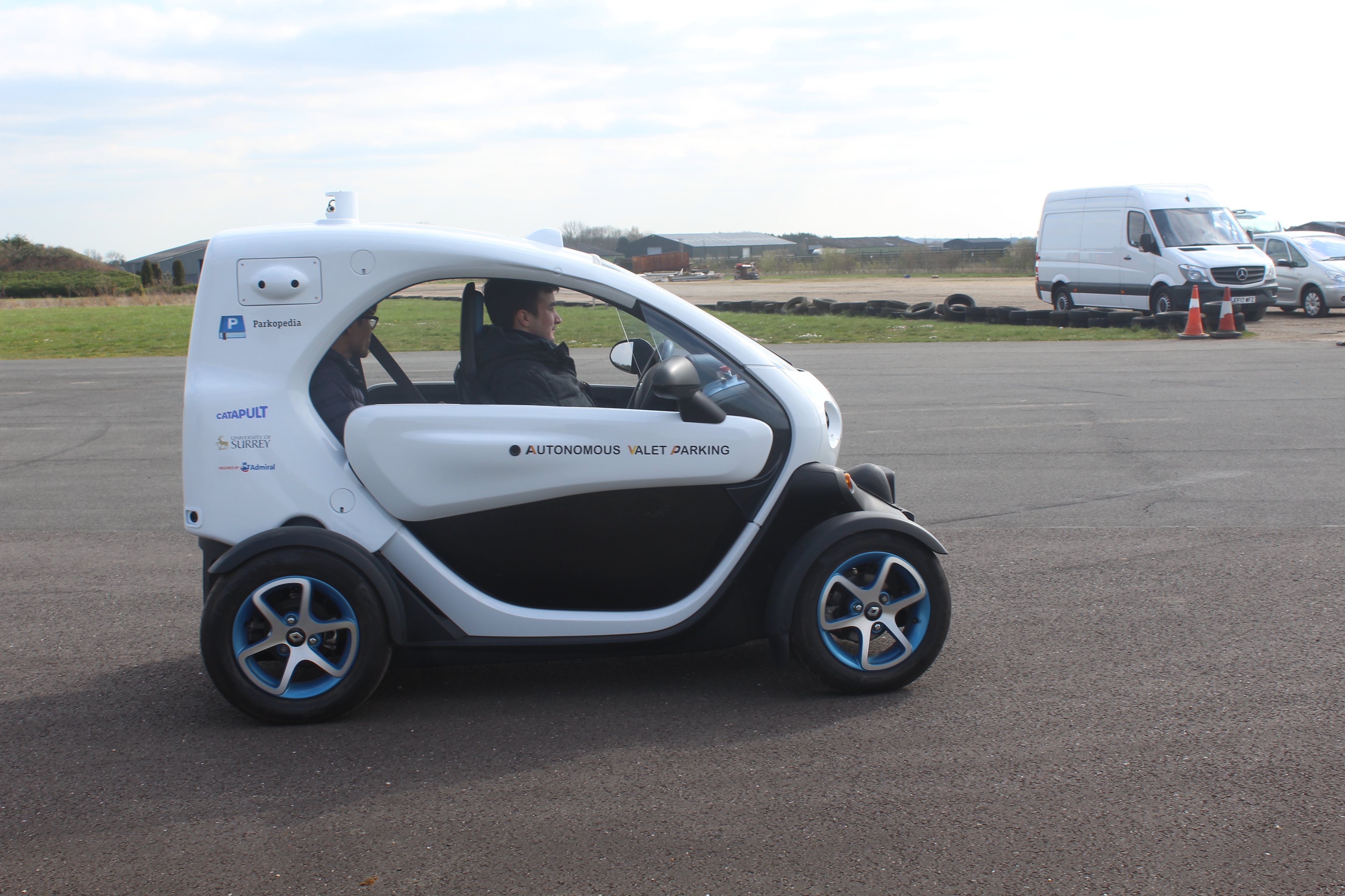
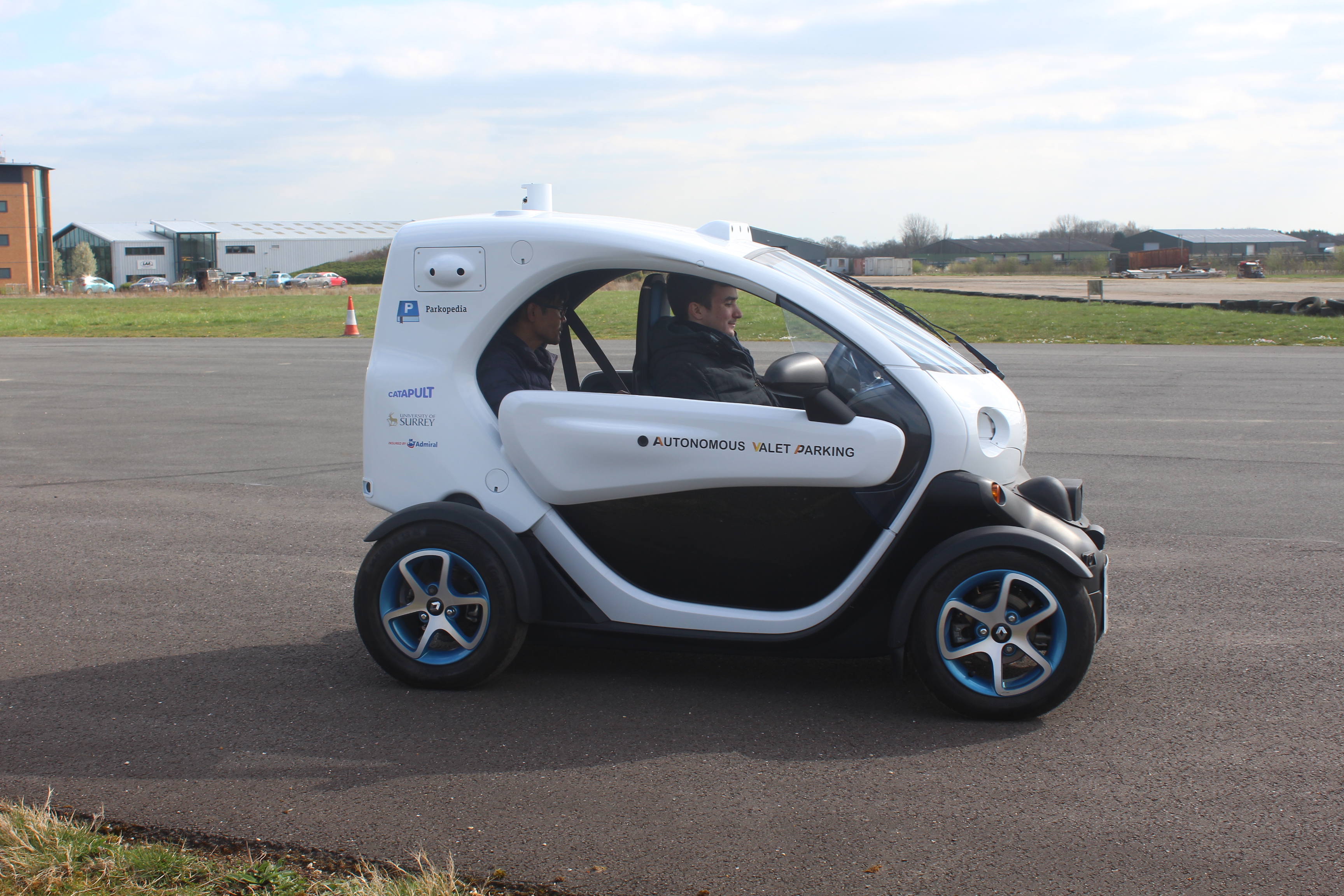
On the final day, we tested a basic path following to make sure everything worked together. We integrated the drive-by-wire (dbw) system with a path follower, PID motion controller and a basic gps and imu localisation in this open space environment.
We managed to achieve the objective of testing the dbw with the feedback control for the path following. However, precision was not there as we expected. The basic imu and gps sensor localisation would not give very accurate positioning and tends to drift away or jump around to within 5m accuracy. To resolve this issue, we are working on a better localisation using RTK GPS (like a simpleRTK2B) using RTK corrections over NTRIP.
Our next test will focus on path following using the high quality localisation and we also hope to start with path planning within the open space. More updates will follow!
Safety is the highest priority at the Autonomous Valet Parking project. As we seek to demonstrate that Parkopedia’s maps are suitable for localisation and navigation within covered car parks, our safety case must ensure the safety of the people, vehicles and infrastructure inside our test vehicle and without. There have been some highly publicised incidents involving other organisations’ autonomous vehicles over the past year or two, so what is the AVP project doing around safety?
Our Safety Case involves a combination of System Safety and Operational Safety, to achieve the required assurance levels around our activities. System Safety covers any and all aspects of the system (hardware, software or both) that contribute to the safety case and is the focus of this post. Operational Safety is all the operational decisions taken to ensure that we are conducting the tests safely and you can read more about that here.
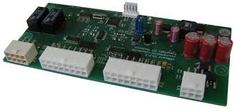
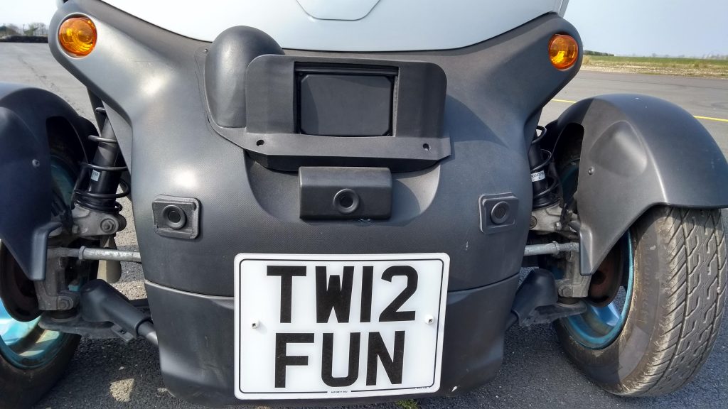
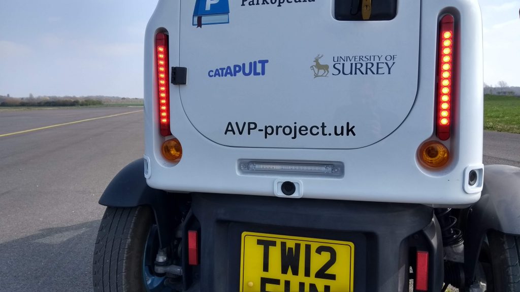
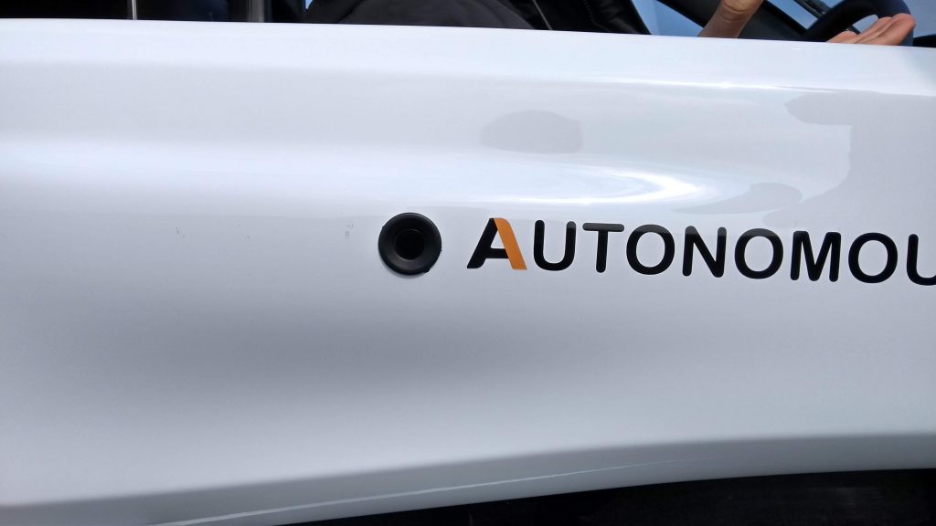
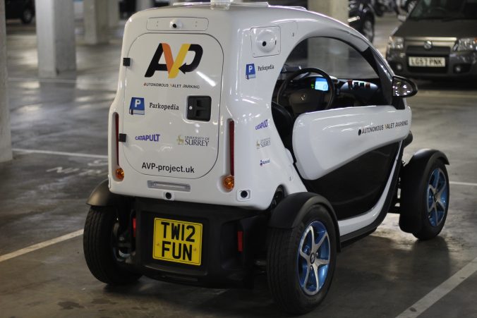
Our test vehicle, a StreetDrone.ONE is a converted Twizy, and comes with ultrasound range sensors. There are eight Neobotix ultrasound sensors in total, three to the front, three to the rear, and one in each door looking sideways. The front sensors are slightly fanned out, and in the rear the outer two are corner mounted. The signals from each sensor are gathered together by a Neobotix board and this publishes the range data as an automotive industry canbus signal. These can be monitored and action taken when a significant measurement is made.
The sensors create a “virtual safety cage”. This virtual safety cage can be imagined as an invisible cuboid around the StreetDrone.ONE, slightly wider and longer than the car itself. If anything, be it a car, pedestrian or wall, intrudes inside this cage, the car should stop immediately, thus acting as a belt and braces to the perception and navigation parts of the AI driving the car.
The video below shows a demonstration of the drive-by-wire system of the StreetDrone at 14 mph. The brake is applied by the actuators at the very beginning of the 3 metres wide white strip. Based on a 14mph start speed, we calculated the braking distance to be 4.5 metres. This is obviously an approximation, and the actual braking distance and time depends on many factors including brake disk wear and tear.
Applying 100% brake at 14mph
Remembering our high-school equations of motion:
Where “v” is the initial velocity, “u” the final velocity, “a” is the acceleration and “s” the distance.
Now we can rearrange this to obtain the acceleration, remembering in our case the final velocity is zero:
These numbers match well with the similar experiments carried out by StreetDrone using IMU data, which have shown peak deceleration of 0.67g and an average deceleration of 0.46g.
The maximum range of the Neobotix ultrasound sensor is 1.5 metres, so we could do the above calculation in reverse and calculate the maximum safe speed. Allowing for a safety buffer of 0.5m:
The distance “s” is 1.0 metres, the acceleration “a” is 4.3m/s^2, and again the final velocity “u” is 0 m/s.
The present AVP plan calls for a maximum speed within car parks of 5 mph which is well within the safety margin calculated above. The next step now is to process the data we’ve captured from the ultrasonic sensors and to develop the software that will automatically apply the maximum brake whenever the virtual safety cage is breached.
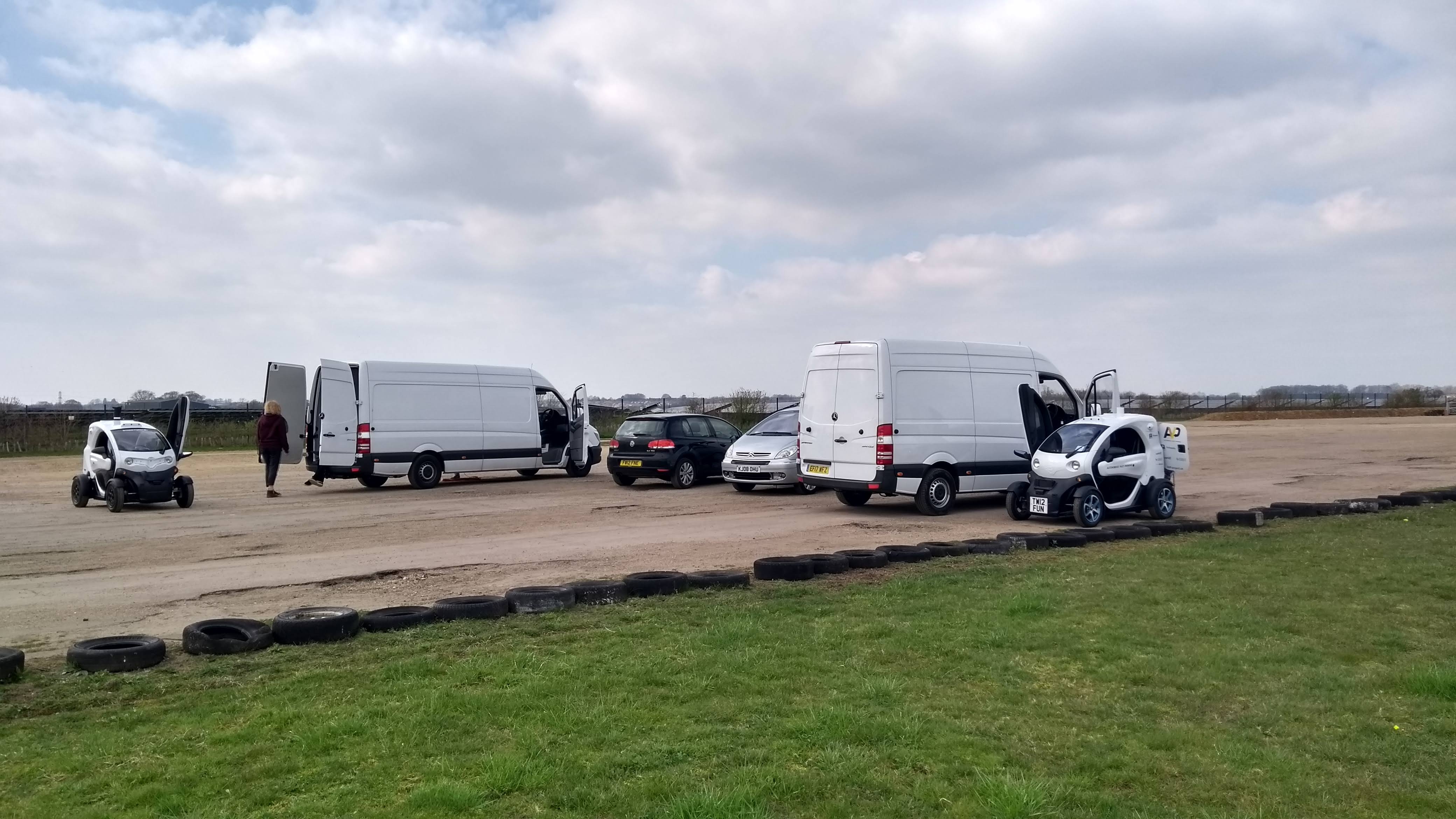
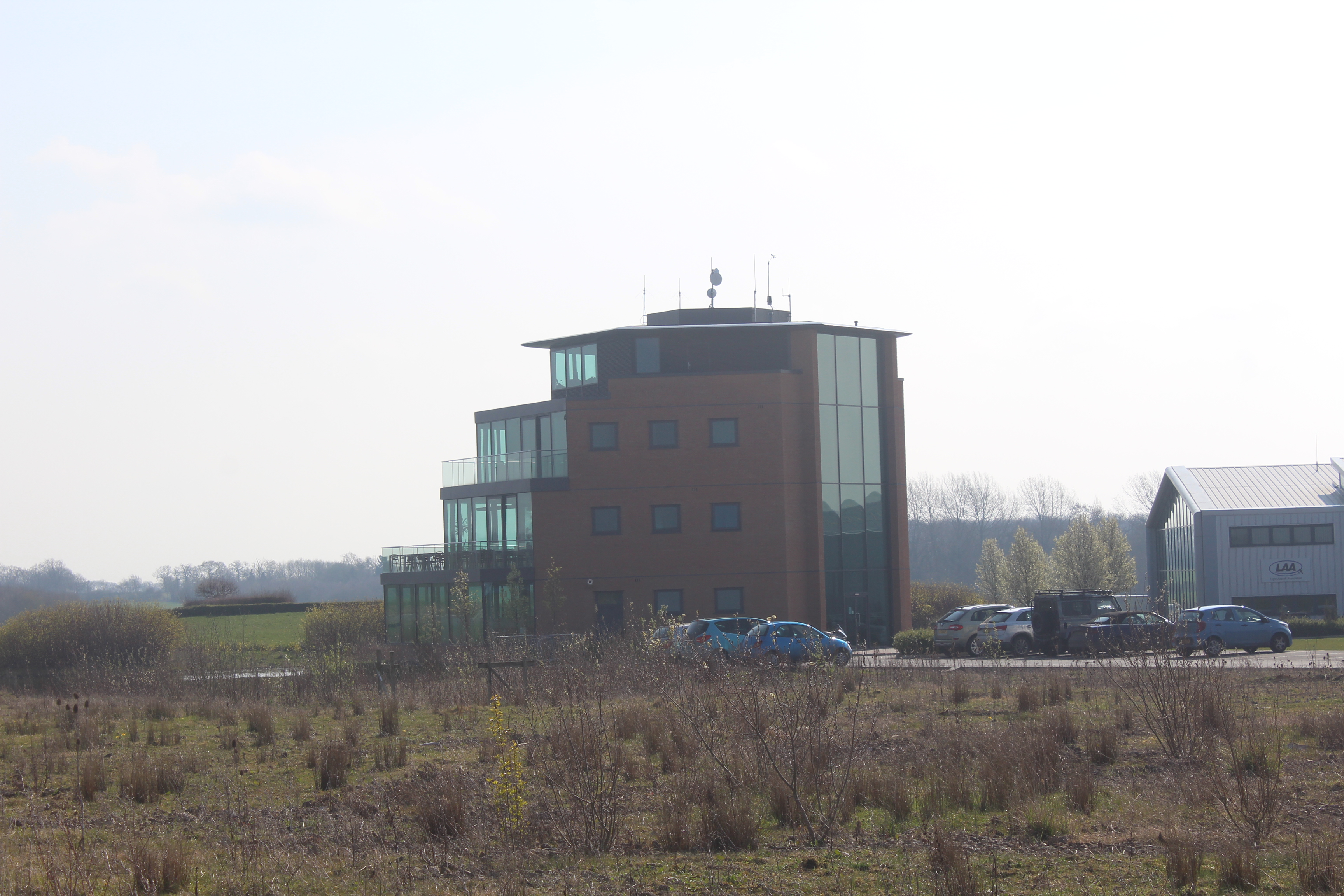
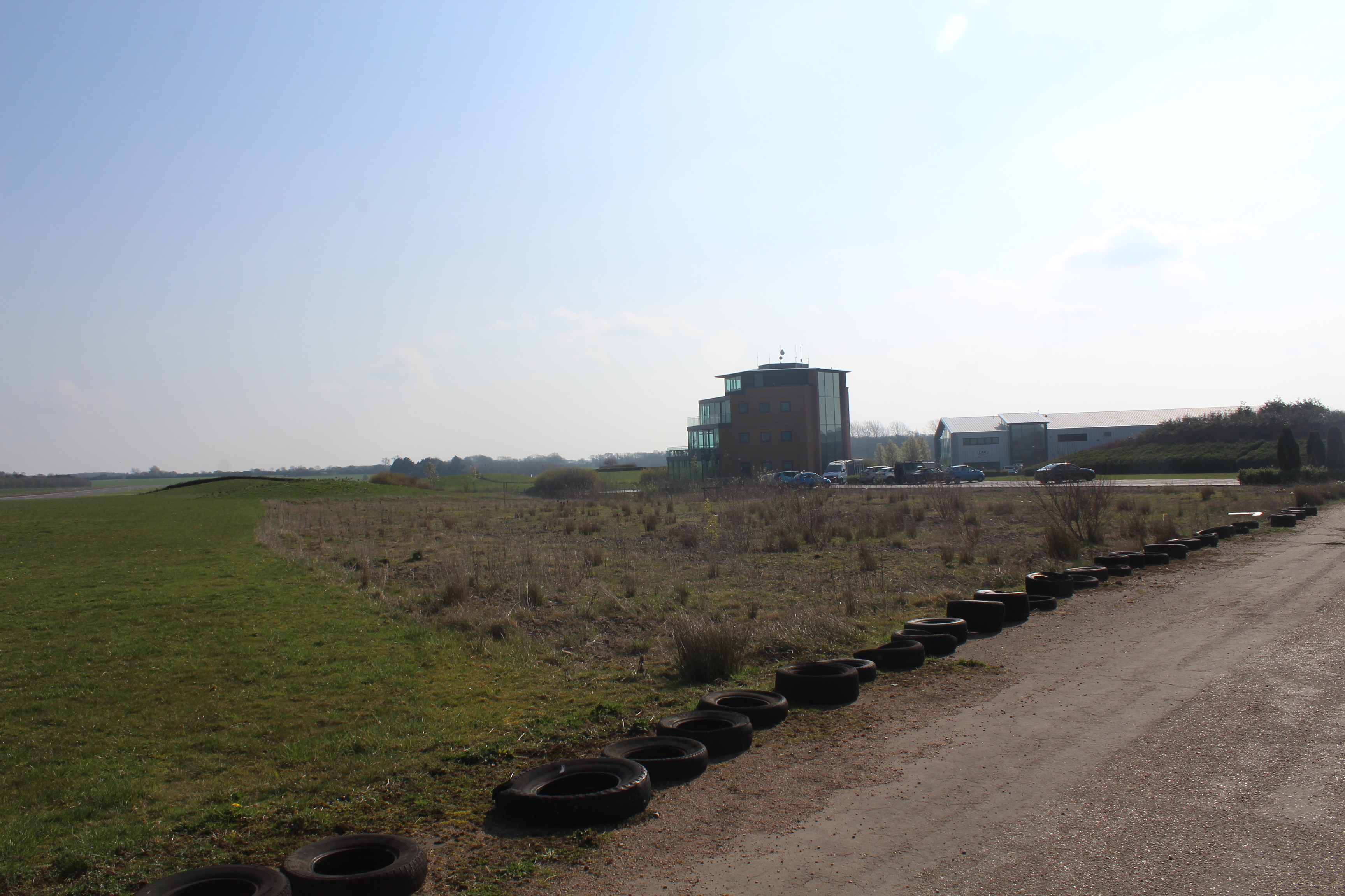
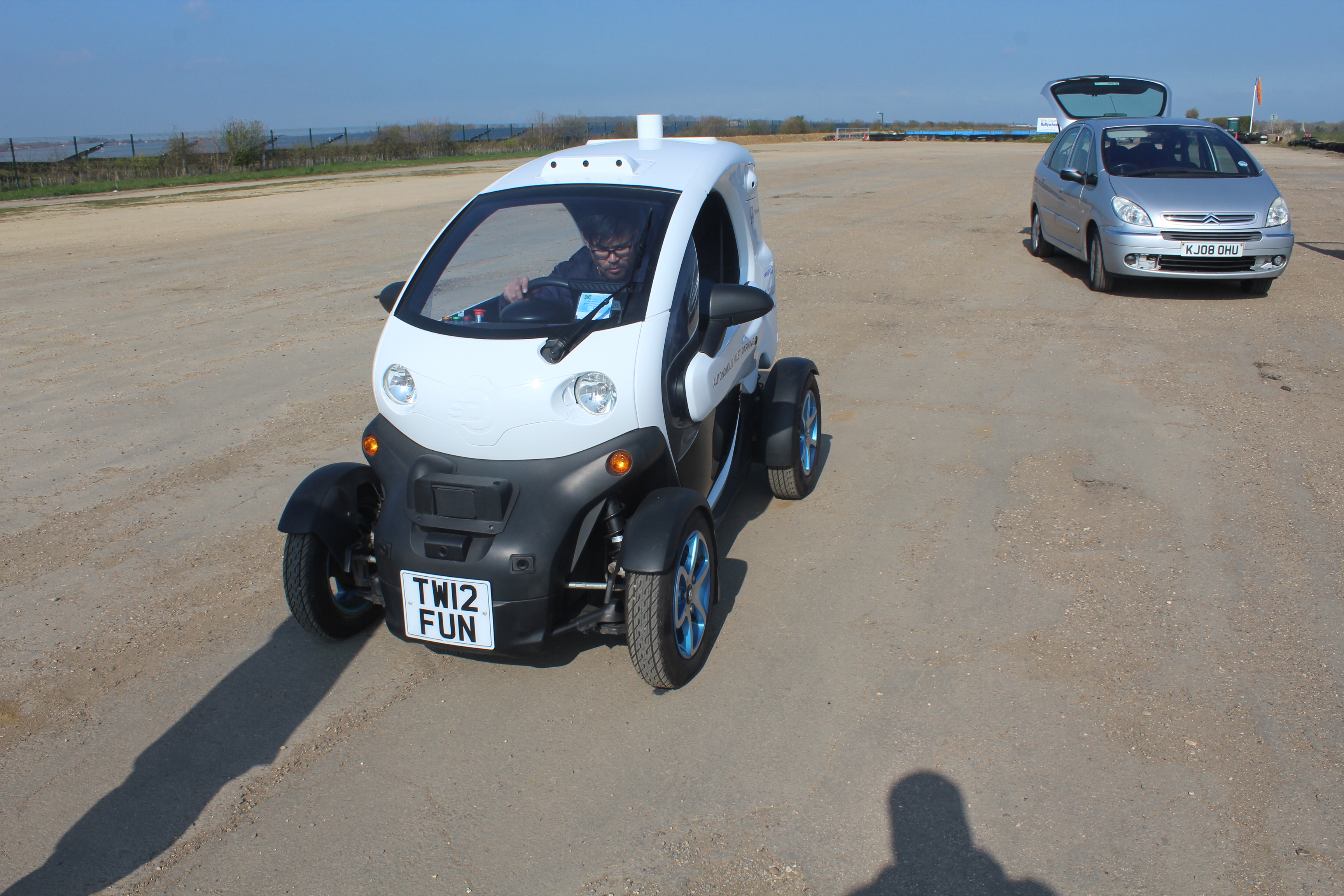
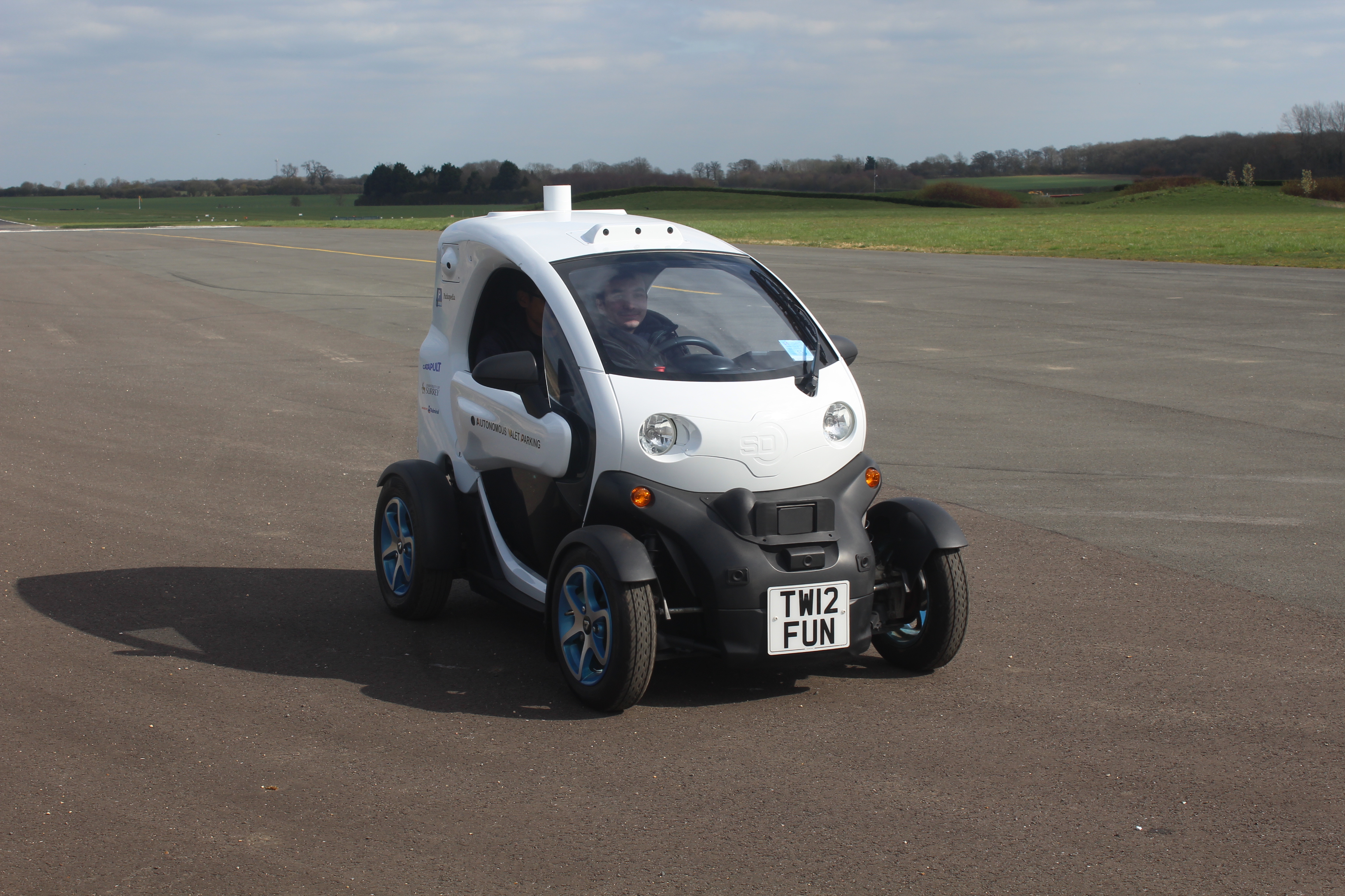
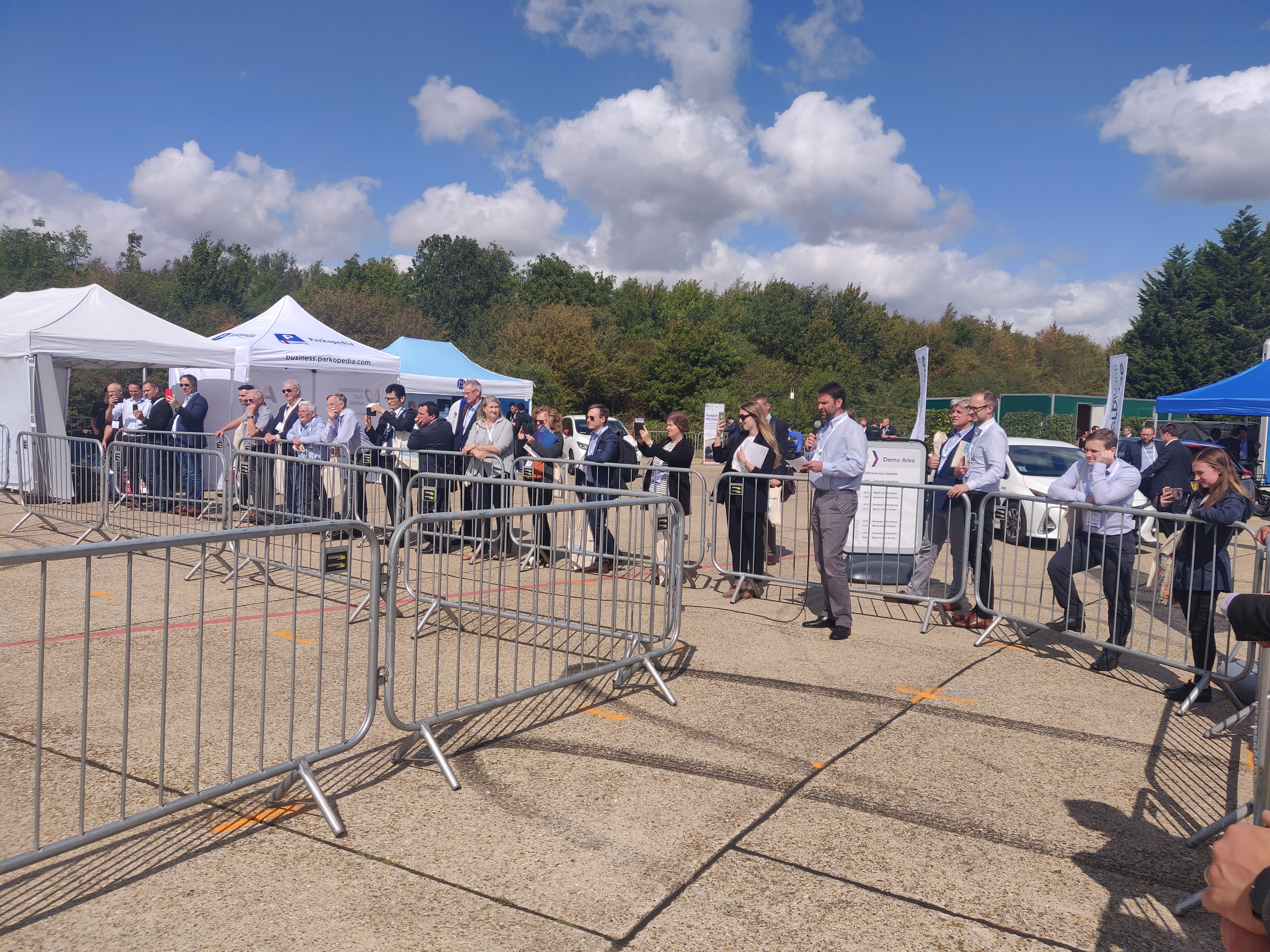
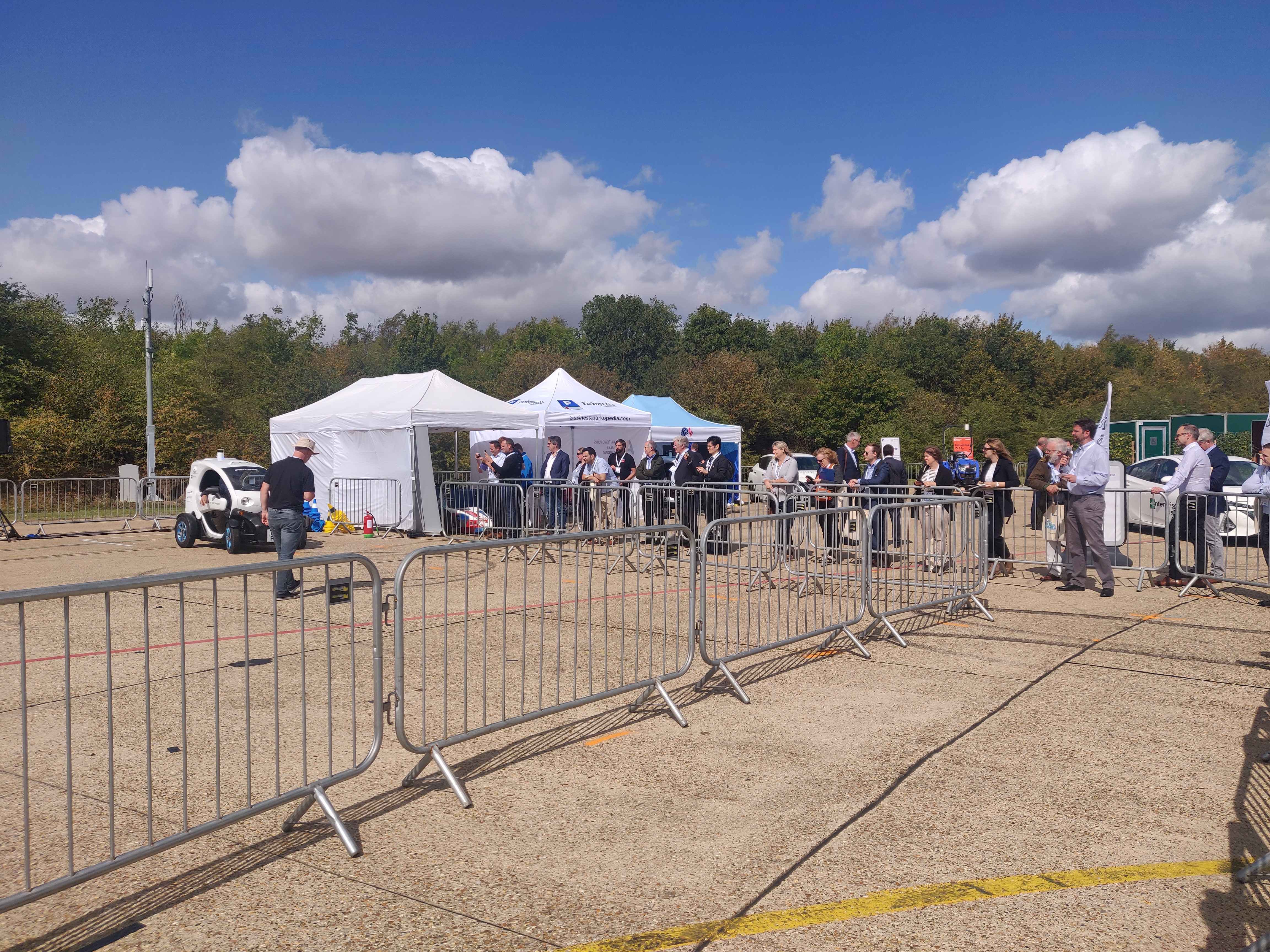
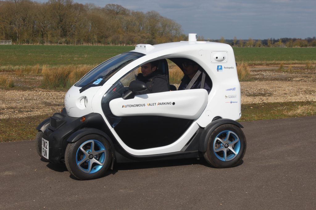
Exciting times: this week marks the start of testing for our StreetDrone autonomous vehicle, as we build towards an Autonomous Valet Parking demonstrator.
This first testing phase will be in a controlled environment to minimise risk. For that reason, we’ve chosen Turweston Flight Centre, which has previously been used by our friends at StreetDrone who have done some of their testing there.
In accordance with our project Safety Plan and the Safety Case for this phase of the project, we’ve also been busy collecting safety evidence prior to starting the live tests. These documents will be made publicly available as part of our goal to be as transparent as possible, and for those who wish to use them as a starting point for their own safety case.
For this phase, our safety evidence documents are:
Why Autonomous Valet Parking, not robo-taxis, will lead the adoption in self-driving technology
Looking back on 2018, the press have reported it to be the year when the hype around self-driving “came crashing down” with the first driverless fatality in March 2018. The first driverless taxi service was rolled out but it didn’t quite have the impact that the industry was expecting.
Research on self-driving cars has been continuing for more than 30 years, starting with the pioneering work by Ernst Dickmanns on the PROMETHEUS project. A lot of work has taken place since then and is still ongoing, but the question remains: why has the problem of self-driving still not been solved in 30 years?
In a sense, the problem has been solved and autonomous driving is already here. Heathrow pods, Greenwich pods, Easymile, May Mobility are live now, and many others are already in production. What sets these simpler systems apart from the systems being developed by Cruise, Argo, Aptiv, Waymo, Uber, Aurora, Lyft, FiveAI and others, is that the environments into which they are deployed are constrained in some way.
The biggest challenge faced by the developers of general purpose self-driving technology is the requirement to handle complex environments with unpredictable interactions. Waymo’s director of engineering recently summarised the challenge by saying that the final 10% of technology development is requiring 10x the effort required for the first 90%. Where the environment is simpler or constrained, then self-driving technology reduces to that of autonomous mobile robots like the kiva.
A more realistic approach to deploying self-driving is therefore needed. The two major places where self-driving car technology are likely to be deployed are on motorways – constrained environments with very strict rules, limitations on cyclists and pedestrians – and low speed restricted environments like retirement villages and car parks.
Autonomous Valet Parking (AVP)
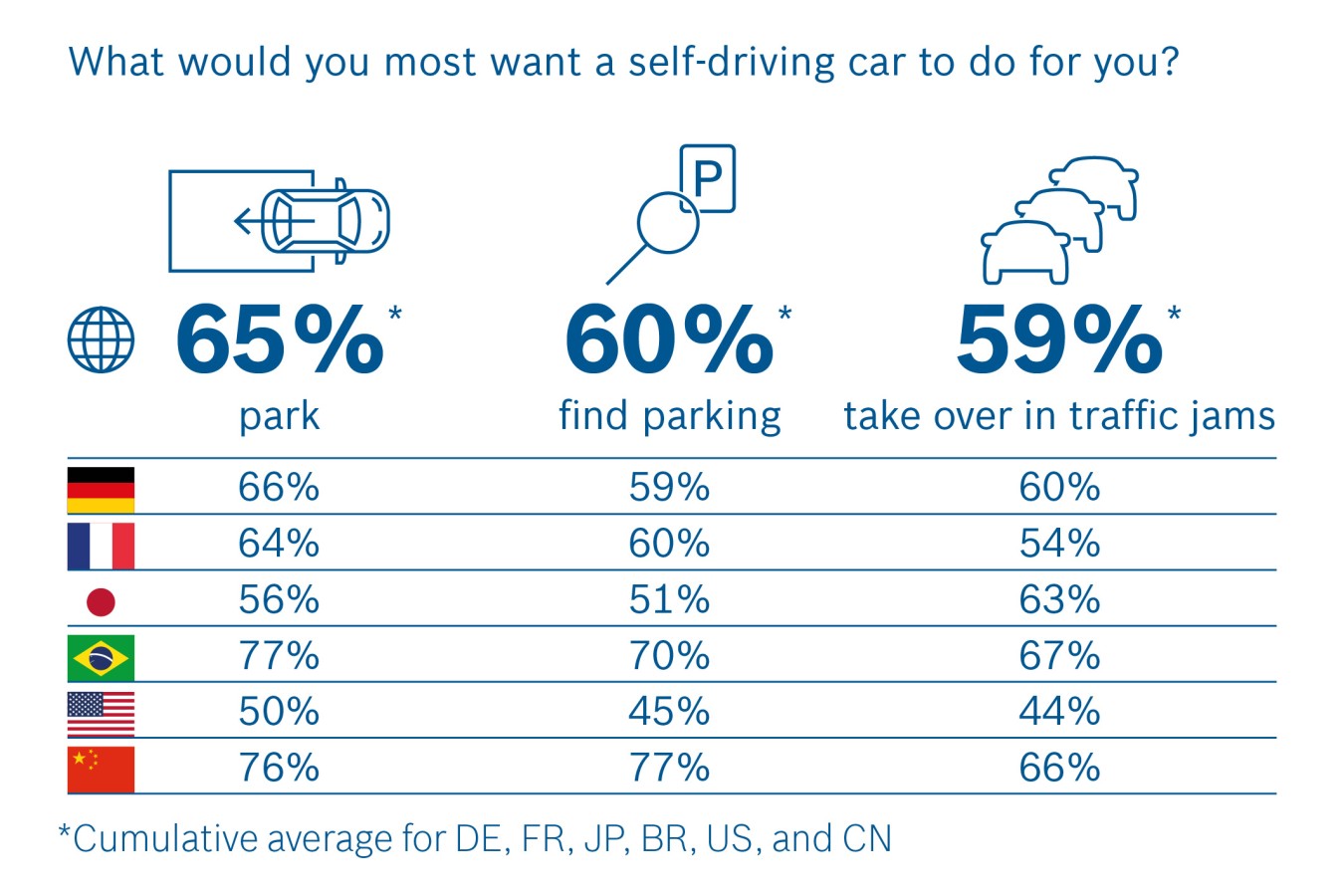
Parking is one of the most important challenges for a traveller, with a parking pain point experienced on 12% of UK journeys (19% in London); the average driver spends 6.45 mins looking for a parking space during each journey. With nearly 1 in 5 journeys already experiencing problem finding a space, AVP represents a way of solving not only the current parking pain point, but also improving the overall parking experience for the other 81% of drivers. BCG’s 2015 report showed that 67% of drivers are interested in “capabilities such as automated searching for parking spots and autonomous valet parking”. Bosch’s 2017 study found that two thirds of consumers want an automated parking feature.
A study by Allensbach in 2016 asking the question “When would you want a driver assistance feature to take over for you?” overwhelmingly showed parking as the most desirable feature.
When German consumers were asked by Bitkom in 2016 when they would be willing to hand over control to the vehicle, the answer similarly was for parking.
The idea of Autonomous Valet Parking is to mimic the Valet function available in selected car parks. After driving to a suitable drop-off location at or near the entrance of the car park, and similar to handing the keys to a valet, the driver presses the “PARK” button on a specially designed app. The car then drives off under autonomous control and finds a suitable place to park. When the driver wants the vehicle back, they will press “SUMMON” and the vehicle will navigate to the pick-up zone.
The Society of Automotive Engineers (SAE) classifies this as a Level 4 feature, in that it provides total automation under specific circumstances.
Based on publicly available information, almost all premium OEMs (Daimler, Audi, JLR, VW, BMW) are working on AVP pilot projects . The reason this feature is so desirable is that it:
Improves the parking experience by allowing drivers to be dropped off at a convenient location (e.g. at the entrance of the car park closest to the desired location such as shops or food court), avoiding the inconvenience and stress of having to find a parking space.
Utilises parking spaces more efficiently by tighter/double parking of autonomous cars, and optimally distributing these vehicles within the available parking real estate.
Avoids unnecessary congestion and pollution through real-time dissemination of parking space availability to the connected autonomous cars.
In addition to the economic benefits, there are clear social and environmental benefits. Driving around looking for parking causes stress and frustration, costs, wasted time, missed appointments, accidents and congestion, noise pollution and CO2 emissions. IBM’s parking survey found that in addition to the typical traffic congestion caused by daily commutes and gridlock from construction and accidents, it is estimated that over 30 percent of traffic in a city is caused by drivers searching for a parking space. By reducing the need to circle looking for a space, AVP has the potential to significantly reduce unnecessary congestion and pollution.
With space at a premium in busy city centres, vehicles equipped with AVP technology could make use of the less desirable spaces that are further from the entrance, freeing up parking spaces closer to a desired destination for those without the technology.
In addition to the economic, social and environmental benefits to AVP, there are also some technical reasons why it is a good candidate feature for large scale public rollout.
1) low speeds mean much lower risk of damage to people, cars and infrastructure.
2) a constrained environment means that the complexity of interactions with other actors has the potential to be significantly reduced.
3) the cost of the required sensor suite and hardware platforms is lower because of the reduced risk and lower speeds.
Conclusion
This consortium’s key objective is to identify obstacles to the full deployment of AVP through the development of a technology demonstrator. It aims to achieve this goal by
Developing automotive-grade indoor parking maps, required for autonomous vehicles to localise and navigate within a multi-storey car park.
Developing the associated localisation algorithms – targeting a minimal sensor set of cameras, ultrasonic sensors and inertial measurement units – that make best use of these maps.
Demonstrating this self-parking technology in a variety of car parks.
Developing the safety case and preparing for in-car-park trials.
Engaging with stakeholders to evaluate perceptions around AVP technology.
Autonomous Valet Parking is a low cost, low risk and high reward feature that consumers want. It makes sense then to expect that this feature will be the first fully autonomous feature (at level 4 or 5) available to the general public. Through Parkopedia’s autonomous valet parking project, we are actively working to make that desire a reality.
Parkopedia’s mission is to improve the world by delivering innovative parking solutions. Our expertise lies within the parking and automotive industries, where we have developed a solid reputation as the leading global provider of high quality off-street and on-street parking services.
Parkopedia helped found the AVP consortium because we believe that Autonomous Valet Parking will become an important way in which we can serve our customers, by reducing the hassle of the parking experience. Parkopedia are providing highly detailed mapping data for off-street car parks, one of the critical components to a car being able to successfully park autonomously.
To make Autonomous Valet Parking a reality, the consortium first selected the StreetDrone.ONE as its car development platform. We are now developing the software stack to run on our StreetDrone with NVIDIA Drive PX2. The University of Surrey, another founding member of the AVP consortium, provides the camera-based localisation algorithms needed for the car to navigate autonomously inside a parking garage, which will support vision, in addition to LiDAR-based localisation.
Parkopedia has joined the Autoware Foundation as a premium founding member, along with StreetDrone, Linaro/96Boards, LG, ARM, Huawei and others. We believe in open source as a force multiplier to build amazing software, and the AVP consortium is committed to using Autoware as the self-driving stack which will run on our StreetDrone and PX2 to demonstrate Autonomous Valet Parking.
Autoware was started in 2015 by Professor Shinpei Kato at the Nagoya University, who presented it at ROSCon 2017. Autoware.ai is based on ROS 1, which has certain fundamental design decisions that make it impractical for production autonomous cars. ROS 2, backed by Open Robotics, Intel, Amazon, Toyota and others, is quickly maturing, and from the very beginning was designed to fulfill the needs of not only researchers in academia, but also the emerging robotics industry.
Autoware.Auto launched in 2018 as an evolution of Autoware.AI, based on ROS 2, applying engineering best practices from the beginning, such as documentation, code coverage and testing, to build a production-ready open-source stack for autonomous driving with the guarantees in robustness and safety that the industry demands. We want to modularise Autoware.ai and align with Autoware.Auto and move to ROS 2.
We want high quality software, we care about safety and we want to do things right. Parkopedia’s main contributions so far have been to improve the quality of the code by fleshing out the CI infrastructure, adding support for cross-compiling for ARM and the NVIDIA Drive PX2, modernising the message interfaces and developing a new driver to support 8 cameras, among other improvements.
Our plan for 2019 is to keep contributing to Autoware.AI and Autoware.Auto to support the StreetDrone ONE and to make whatever changes necessary to support our Autonomous Valet Parking demonstration.
We’re very grateful to Shinpei Kato and the Tier4 team for open-sourcing Autoware and for welcoming our contributions.
One of the key objectives of this Autonomous Valet Parking project is to demonstrate our autonomous vehicle parking itself in a covered car park. The Transport Systems Catapult is responsible for the safety work package which ensures that all activities undertaken during the project are done in a systematic and safe manner. One of the important deliverables to ensure safety is the Risk Assessment and Method Statement (RAMS).
The RAMS document generally includes:
1. An overview of the project and key objectives to provide the reader with a background of the project
2. The activity being assessed, including:
Roles and responsibilities
Limits of the operation and trial details (route planned, scenarios, vehicle specifications, time of day, limits, weather, specifications)
Legal considerations such as vehicle insurance and laws
Training achieved (eg. driver training on the StreetDrone.ONE vehicle, taking over manually)
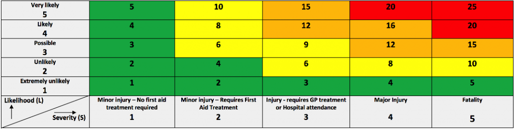
3. A risk assessment listing hazards, consequences, mitigation methods and detailing who might be harmed. Following the ISO 26262 standard, a hazard analysis and risk assessment is required in order to determine the criticality of a system.
The risk analysis is focused on:
Risks related to the ongoing operation of the vehicle
Risks related to the operation of external factors that affect current operation
Risks arising from the new equipment that may affect the safety of the vehicle or other
RISK MATRIX (To generate the risk level)ACTION LEVEL (To identify what action needs to be taken)
The method statement part describes in a logical sequence how a task will be carried out in a safe manner. It includes all the risks identified and the measures needed to control those risks.
The purpose of the method statement is to ensure that:
The trial is carried in a structured, controlled and safe manner
The hazards and associated risks are understood and mitigated
While the ultimate goal of the project is to demonstrate Autonomous Valet Parking, we will build up to this demonstration through smaller manageable steps and a separate RAMS will be produced at each stage:
At Parkopedia’s Autonomous Valet Parking team, we will be creating indoor car park maps for autonomous vehicles. Throughout this 2.5 year project, in collaboration with Transport System Catapult and the University of Surrey, we expect to be doing a significant amount of deep learning. We estimate that over the course of this project there will be intensive training on large datasets, for multiple days, weeks or even more. As any deep learning project there are three distinct phases in the research and development pipeline, which can be loosely described as (1) prototyping; (2) hyperparameter search and (3) intensive training. While there will be a lot of prototyping involved, which we believe any high-end desktop computer equipped with one GTX Nvidia 1080 Ti will fit our needs, the next question is how do we efficiently solve (2) and (3). Typically, in (2) one picks different parameters of the model and trains it against the dataset (or part of it) for a few iterations. In our case, a reasonable estimate could be perhaps 10 different runs, each taking a day of processing time. This insight (best hyperparameters) is then used to apply heavy computation in (3).
We are at the early stages of this project, but due to accounting reasons, we need to have a clear vision now on where we want to apply the budget for computing power for deep learning. Given that we know beforehand that we’ll need to have it for a relatively long period and we will do a lot of experimentation on large amounts of data, we want to investigate what is the most cost effective solution. On the other hand, because of the high processing times involved, it is important that the solution has enough flexibility to the research team, in that heavy computation times don’t hinder the ability to focus on other tasks that might require a GPU too. This blog post is about finding the sweet spot between these two.
The discussion is generally around on-premise hardware vs cloud based solutions. A cloud based solution is appealing because resources are readily available, maintenance-free, and one can launch as many computing machines as desired at any point in time. This flexibility also has a much wider hardware choice: a multitude of flavours are available so one is not restricted to working with a certain hardware architecture. Of course, these very interesting features come with a price. Whilst an office-based solution doesn’t offer these characteristics, it is interesting to see how they compare, especially in the long run. Therefore, it comes down to asking the following question:
What infrastructure gives us the best compromise between time-to-solution, cost-to-solution and availability of the resources ?
The goal of this document is to do a performance vs cost study on different possible architectures, both cloud-based and office-based. We ran benchmarks on various AWS GPU instances, and extrapolated some of the results to other similar cloud based architectures on Google Cloud. We compared the results against a system with 4 Nvidia GTX 1080 Tis, by extrapolating the results obtained for a single GTX 1080 Ti, which we currently have. An analysis was made both in terms of performance and cost.
2. Experimental Setup
We ran the tensorflow benchmark code repository which according to their description, “contains implementations of several popular convolutional models, and is designed to be as fast as possible. tf_cnn_benchmarks supports both running on a single machine or running in distributed mode across multiple hosts.”, which is perfect for running it against various infrastructures, both in single and multiple GPU scenarios. In terms of software all the infractures had the exact same configuration, namely:
Cudnn 7.1.4
Cuda 9.0
Python 2.7
Ubuntu 16.04
2.1. Amazon Web Services (AWS)
Amazon’s GPU options are very simple: you choose an instance which comes with one (or more) GPUs of any given type. We compared three GPU families on AWS p2s (K80s), g3s (M60s) and p3s (V100s).
Gpu
Instance
#GPUs
On demand price $/hour
1 day
1 week
1 month
NVIDIA K80
p2.xlarge
1
0.9
21.6
151.2
658.8
p2.8xlarge
8
7.2
172.8
1209.6
5270.4
p2.16xlarge
16
14.4
345.6
2419.2
10540.8
Tesla M60
g3.4xlarge
1
1.14
27.36
191.52
834.48
g3.8xlarge
2
2.28
54.72
383.04
1668.96
g3.16xlarge
4
4.56
109.44
766.08
3337.92
NVIDIA V100
p3.2xlarge
1
3.06
73.44
514.08
2239.92
p3.8xlarge
4
12.24
293.76
2056.32
8959.68
p3.16xlarge
8
24.48
587.52
4112.64
17919.36
2.2. EC2 Spot Instances
Spot instances are a solution offered by Amazon’s EC2, which defines it as an: “(…) unused EC2 instance that is available for less than the On-Demand price. Because Spot Instances enable you to request unused EC2 instances at steep discounts, you can lower your Amazon EC2 costs significantly (…)”. One thing to have in mind is that its pricing scheme is based on offer/demand model, resulting in a fluctuant hourly rate. In a nutshell, the user selects the hardware (say p3.2xlarge), defines how much he/she is willing to pay per hour, and the machine is accessible, provided the price set is below AWS’ price threshold. In such an event, the machine is automatically shutdown by Amazon. On the financial side, this is obviously very appealing as one gets the same hardware for a fraction of the cost. However, on the technical side, this solution requires a more complex architecture, which can handle interruptions (on a DL scenario this means most likely saving the network’s weights and gradients often to a location outside the local instance). The user must also accept downtimes – even if there is an orchestration mechanism that automatically launches on-demand instances to recover the loss of an instance and continue training/inference, there’s an initialization stage (setting up the instance, downloading the last state of the network, downloading the dataset, etc) – that cannot be ignored. Moreover, there’s a considerable effort in coming up with such orchestration mechanism, which cannot be disregarded as well, as it brings to advantages to the deep learning researcher; in fact, it’s quite the opposite.
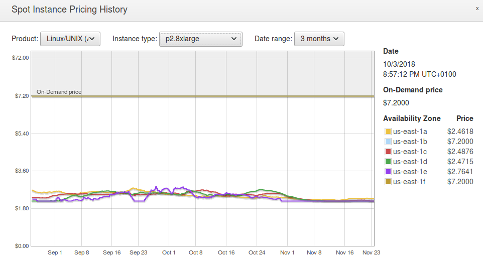
Because of these reasons, this solution doesn’t directly compare with the two main solutions in debate. Nevertheless, we believe that in order to have a more balanced post, it should be added here. Below is a screenshot of the last 3 months obtained from AWS’ EC2 Management Console for a p2.8xlarge instance.
In order to work out an hourly rate for EC2 spot instances, we’ve taken the cheapest curve for all the availability zones, and we came up with a ballpark estimate for its average price throughout the 3 months period. The following table summarizes this information for all the instances, as well as the discount with respect to the on demand prices.
Spot price
$/hour
Cost
wrt on-demand
p2.xlarge
0.28
31%
p2.8xlarge
2.71
38%
p2.16xlarge
5.32
37%
g3.4xlarge
0.37
32%
g3.8xlarge
0.68
30%
g3.16xlarge
1.37
30%
p3.2xlarge
1.11
36%
p3.8xlarge
4.85
40%
p3.16xlarge
8.00
33%
2.2. Office GPU box
For a proper comparison against cloud-based solutions, we need to come up with an hourly rate for the office GPU. Working out the equivalent price/hour involves making assumptions on the utilization (the more we use it, the cheaper it becomes, per hour). In addition to the hardware acquisition, we want a maintenance contract. This is because we want to minimize downtimes when a certain GPU goes out of order temporarily (unfortunately, it is not that unusual, and is in itself a disadvantage of this solution). Because this project will run for 30 months, we can amortize this price per month and depending on the average utilization in terms of the number of days the box is used (24 hours per day, uninterruptedly), we can reach a final figure for the hourly rate. To be even fairer, one might consider adding in the electricity costs, which we thought it would make sense.
Broadly speaking, in our scenario, a box of 4 x GTX 1080 Ti (about $6.5k USD with a maintenance contract), assuming 20 USD cents per kwh in the UK, being used 10 days per month equates into about $1.30/hour. We appreciate this 10 days is a strong assumption, especially in this early stages of the project. Therefore we test different utilization figures later. A breakdown of this figures is shown below:
Cost estimation of office GPUs
Hardware
Box (4*1080tis)
$6,500.00
w/ 5 Year Warranty, 3 Years Collect & Return
Total Acquisition Cost
$6,500.00
Amortization
Months (length of project)
30
Price / month
$216.67
Electricity
Price per kwh
0.2
Utilization (days per month running 24/7)
10
Cost / month
$48.00
Global cost / month
$264.67
Cost/hour
(assuming previous utilization)
1.10
2.3. Google Compute Engine (GCE)
Google Cloud’s model is slightly different than AWS’ model, in that GPUs are attached to an instance, so one can combine a certain GPU with different host characteristics. As per Google Cloud’s pricing page: “Each GPU adds to the cost of your instance in addition to the cost of the machine type”. We did not run any benchmarks on google cloud, but because their prices are different we thought it would make sense to add GCE’s scenario. Because of this, we only took into account hardware setups that would be comparable to the AWS’ offer, in terms of the GPUs.
Their GPU offering for GPUs consists on the following boards: NVIDIA Tesla V100, NVIDIA Tesla K80 and NVIDIA Tesla P100. The latter was discarded as there’s no counterpart on aws. Also, regarding the K80’s one can only select 1,2,4 and 8 GPUs and as for the NVIDIA V100’s, only 1 or 8 GPUs can be selected
In order to obtain a similar instance to those in AWS, we selected the “base instances” so that the number of vCPUs is the same, as follows:
Alias
Instance
GPUs
Price/h ($) [first term is the instance price/h]
Equivalent aws instance
GCE_1xV100
n1-standard-8
1xV100
0.38+2.48 = 2.86
p3.2xlarge
GCE_8xV100
n1-standard-64
8xV100
3.04+8*2.48 = 22.88
p3.16xlarge
GCE_1xK80
n1-standard-4
1xK80
0.04+0.45 = 0.49
p2.xlarge
GCE_8xK80
n1-standard-32
8xK80
1.52+8*0.45 = 5.12
p2.8xlarge
In terms of performance benchmarks, Tensorflow has done this comparison already. Amazon’s p2.8xlarge was compared against a similar instance, which we denote as GCE_8xK80. Although there appears to be a minor difference, the results are approximately similar, as expected. In our context, we believe we can safely assume the same for the three remaining cases, so we simply used the same performance metrics.
We also took Google TPUs into account. This blog post compared AWS’ p3.8xlarge against a cloud TPU. They show that on ResNet50 with a batch size of 1024 (the recommended size by Google), the TPU device is slightly faster, but slower at any other smaller batch size. We omitted this fact, and used our measurements obtained on the p3.8xlarge.
3. Performance Results
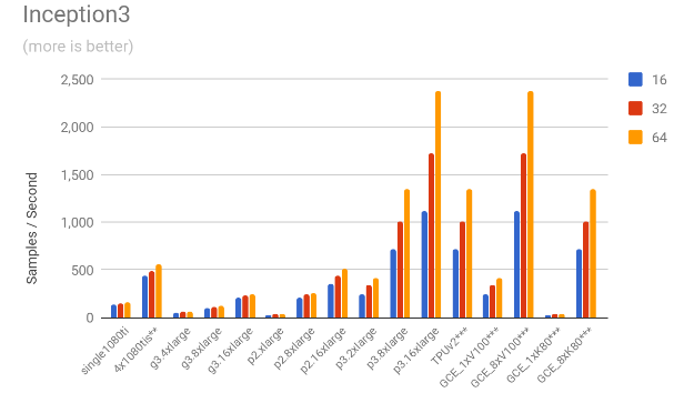
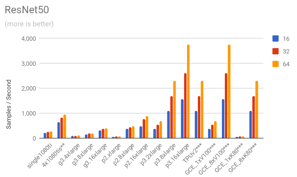
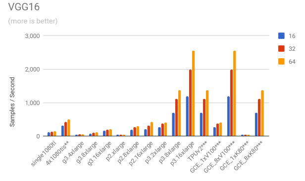
We ran the benchmark code in three different standard models (Inception3, VGG16 and ResNet50) using three different batch sizes per GPU: 16, 32 and 64, meaning that in a multi-GPU training session the effective global number of images per batch is #GPUs x batch size. Half-precision computation was used. A typical command line call would look like this:
As per TensorFlow’s performance guide, “obtaining optimal performance on multi-GPUs is a challenge” […] “How each tower gets the updated variables and how the gradients are applied has an impact on the performance, scaling, and convergence of the mode”. As mentioned earlier, the goal of this analysis is to obtain a ballpark estimate on cloud vs on-premise in terms of performance and cost, so gpu-related optimization issues, are out of scope of this post (this issue has been addressed in various other blog posts, e.g. see: Towards Efficient Multi-GPU Training in Keras with TensorFlow). That said, when we ran the benchmarking code with its default configuration (as show in the python command above), we soon realised we were having poor scalability in terms of throughput, i.e. the throughput didn’t scale well with the number of GPUs, so that wouldn’t be a fair comparison in a more optimized scenario. After reading Tensorflow’s tips, and a bit of experimentation we reached a setup which we were happy with. Note also that using different gpu optimizations might have an impact on training convergence, but we will ignore that for the remainder of this post. Despite this, we only fined-tuned g3.16xlarge and p2.16xlarge and p3.16xlarge instances, which was where the scalability issues were seriously being noted. Note that we don’t claim this to be by any means the optimum configuration, nor did we put serious efforts in it, but it allows us to make a more coherent comparison. The table below shows the scaling efficiency obtained after optimizing each of the three multi-GPU instances, with respect to the respective instance that has a single GPU. For each configuration (AWS instance / model ) the associated letter (A, B, C, x ) refers to the configuration in use, as follows:
A : variable_update:replicated | nccl:no | local_parameter_device:cpu
B : variable_update:replicated | nccl:yes | local_parameter_device:gpu
C : variable_update:replicated | nccl:no | local_parameter_device:gpu
x - default configuration
Inception3
ResNet50
VGG16
#GPU
Config
16
32
64
16
32
64
16
32
64
2
g3.4xlarge -> g3.8xlarge
x
0.94
0.96
0.97
x
0.93
0.95
0.97
x
0.84
0.89
0.93
4
g3.4xlarge -> g3.16xlarge
A
0.94
0.96
0.96
A
0.92
0.96
0.97
B
0.87
0.92
0.93
8
p2.xlarge -> p2.8xlarge
x
0.90
0.88
0.87
x
0.89
0.89
0.90
x
0.70
0.87
0.92
16
p2.xlarge -> p2.16xlarge
C
0.74
0.81
0.86
A
0.58
0.77
0.84
C
0.39
0.52
0.64
4
p3.2xlarge -> p3.8xlarge
x
0.72
0.75
0.81
x
0.73
0.78
0.83
x
0.65
0.74
0.83
8
p3.2xlarge -> p3.16xlarge
B
0.57
0.64
0.72
B
0.53
0.60
0.68
B
0.55
0.66
0.78
Average
0.80
0.83
0.87
0.76
0.83
0.87
0.67
0.77
0.84
In the perfect world these numbers would all be close to 1.0, showing a perfectly linear efficiency in terms of performance as the number of GPUs scale from 1 to many. This table shows that scaling is not perfect but some setups can get quite close.
As mentioned in the introduction, we have one GTX 1080 Ti where we can run these tests on, therefore we had to estimate the performance figures on a box with four of these GPUs. We simply used the average obtained in the earlier table for each of the datasets and batch sizes (see row in red). We believed this to be a relatively conservative estimate. These are the figures obtained.
Inception3
ResNet50
VGG16
16
32
64
16
32
64
16
32
64
1×1080 Ti
136
145
160
213
250
273
118
137
149
4×1080 Tis**
435
482
556
649
825
947
314
418
498
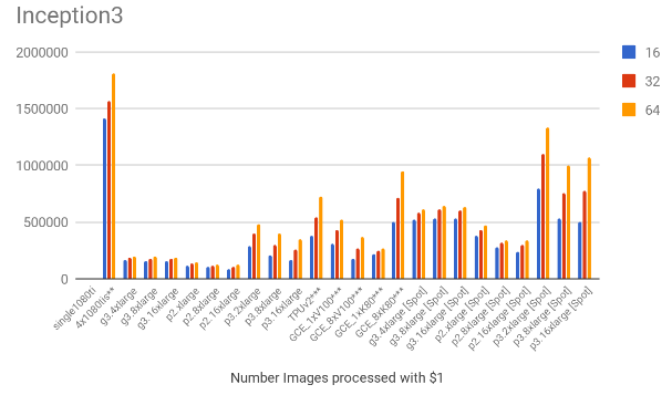
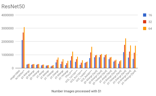
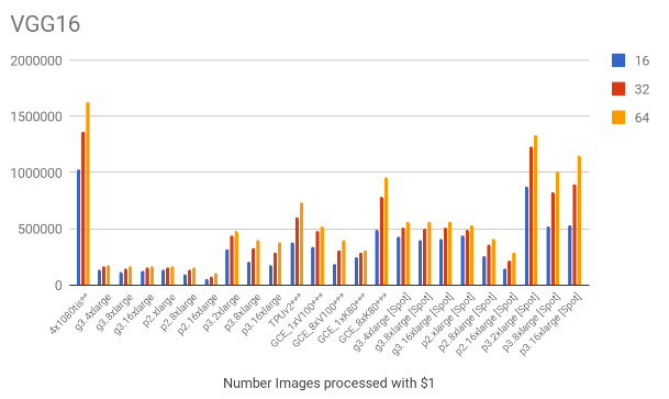
3.1. Throughput comparison
The following charts show the samples / second for each of the models for all the mentioned scenarios.
4. Cost results
Based on the throughput and the hourly costs we can estimate the number of images we can process with $1, which is shown below. Note that the EC2 spot prices were also included on these charts.
5. Additional Comparisons
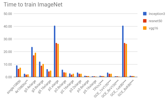
5.1. ILSVRC
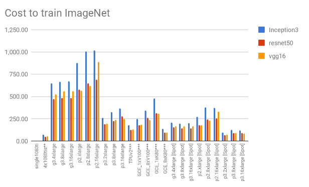
We don’t know yet the amount of data we will be processing, so we thought the ImageNet dataset would be a good choice to give us some real-world intuition on what to expect in terms of time to train and global cost in dollars, as it is pretty much the “industry standard” in deep learning and also because of its respectful size. For each of the models, we their respective papers give us the batch size and the number of iterations, which allows us to work out the total number of samples seen when training.
To estimate these figures, we simply used the cost and time for a batch of 64 for all the models. Note however that in reality the figures would be lower (both for the time and consequently, the cost). This is because we are using a smaller batch size in our estimations, so a better utilisation of the GPU memory (bigger batch size) would increase the performance, so this is just for illustration purposes. Of course, this choice would impact convergence, but we’re disregarding that too.
The two charts below shows us the cost and time to train. Considering only “persistent” solutions (all except EC2 Spot instances), the office-based solution offers a much cheaper solution – almost 2x cheaper than the Google’s GCE_8xK80 (the cheapest persistent cloud-based solution). It is still about 36% cheaper than the cheapest solution on the “spot instances” model. Another interesting fact is that it is the forth best performing solution in terms of time to train.
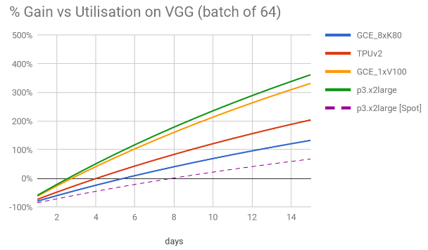
5.2. Gain vs utilization
On previous estimates, we were using an utilisation figure of 10 days – running the box on average 240h per month. As this is just a guess, it is interesting to know how much do we gain (or lose) as we change the number of days per month when compared to a cloud-based solution. To simplify we’ve compared different utilisations against the three best scenarios on VGG16 (64). Again, by doing this comparison on VGG16, is itself a conservative choice, as out of all the models, VGG16 is the one where the images/cost gain of 4x1080tis versus the second best scenario (GCE_8xK80) is smaller – it is better by only approximately 1.7x versus 1.9x on ResNet50 and Inception3, on batch sizes of 64. The comparison is shown on the chart below.
Out of all the the persistent solutions, Google’s GCE_8xK80 is clearly the one with the best value for money. Yet, after 5 days of usage per month, the office GPU outbids Google’s all other cloud based instances. After about 8.5 days per month the box is twice as cheap as TPUv2 – 1.8x and 1.9x respectively for p3.x2large and p3.8xlarge instances. This increases slightly to 10 days for GCE_8xK80. The cheapest spot instance price get outbid only after 8 days of continuous usage.
6. Closing remarks
We believe that throughout our analysis, we were highly conservative in the estimates for an office GPU machine. Essentially, when assumptions had to be made, we tried to compare an office based solution against worst performing scenarios. An accurate estimate depends a lot on the actual scenario but here we tried to be slightly pessimistic with regards to an office based solution.
What we believe matters most is the time and cost to reach a certain solution and our analysis on ILSVRC shows that the 4xGTX1080tis lies perfectly on the sweet spot between these two factors. Another interesting angle is the utilisation chart which clearly shows that, if a GPU box will be used for slightly more than 5 days per month, then cost wise, the on-premise solution is the clear winner. So, on long projects such as the one we’re about to embark, an office based solution is a no-brainer. Therefore the choice is mostly obvious if you need to use GPUs extensively.
Nethertheless, we would like to highlight the following points:
In terms of costs, when compared to AWS, Google’s cloud GPU offering is worth investigating.
We are mindful EC2 spot instances are very appealing, but we believe this scenario didn’t fit our purposes because to gain the value from spot instances a maximum price needs to be set and the job will be terminated if that threshold is breached. Even if it its drawbacks can be surpassed using additional logic to handle the termination and re-start of instances gracefully, we believe such configuration is non-optimal and wouldn’t be appropriate for us.
Another point for consideration regarding EC2 spot prices is that although this analysis was done over a relatively long period of 3 months, effectively reducing the fluctuations, there’s no guarantee cost will stay more or less fixed in the future. In the best scenario it can even be lower, but predictability is required in when budgeting for a 2.5 year project.


Recent Comments